Part III: User Guide – Advanced Functions
7 Advanced Functions and Tools in MSiReader (MSI and BioPharma Modes)
There are a significant number of advanced functions and tools for MSI mode as well as the BioPharma mode (§8) in MSiReader. MSI Software Solutions, LLC is constantly evolving the software to add new features, tools and functions to MSiReader. If you have a suggestion for improvement of existing tools, a request for a new tool, or if you need a customized solution for your research, please email us at support@msireader.com.
Make sure to go to §6 for the basic functions and tools in MSiReader. The description of these is not repeated here.
7.1 Loading Native File Formats from Different Vendors in MSI Mode
The imzML has been very useful in standardizing the field allowing users to convert their data in a two-step process into this format. However, for large projects, experiments with unique data structures, etc. it can be tedious to convert all the files. To this end, in the paid version of MSiReader, we are adding the ability to load native file formats. Once loaded and a user carries out operations on the data, it can then be saved as a *.mss or a *.mim file format that can be used solely in MSiReader and it will load much faster than the original native data file. Please see §3.7 for more information.
There are many different types of data collection in mass spectrometry imaging including, but not limited to, rectangular ROI in flyback or meander mode and arbitrary ROI in flyback or meander mode which requires a location file. The MSI Mode includes information regarding reading native file formats in MSiReader (other formats were described in detail in §3). Moreover, there are many different experimental workflows for HTS/HCS and thus, we have included these different ways to read in these types of data (§8.2) for both imzML and *.raw files. Each scenario has been implemented in MSiReader.
7.1.1 Loading Thermo Fisher Scientific *.raw files in MSI Mode
The simplest data collection of mass spectrometry imaging data is a rectangular ROI where the user must know the following information: spots per line, number of lines (the product of these two numbers is the total number of scans), spot spacing and line spacing, and whether they were collected in meander or flyback mode. There is a test dataset online under Thermo RAW and then subfolder Rectangular ROI for testing this feature. More advanced data collection strategies such as Arbitrary ROI, requires a location file. For the Arbitrary ROI, test data are provided with a location file in Arbitrary ROI subfolder. Both of these scenarios are described in the next two sections.
7.1.1.1 Loading a *.raw file with Rectangular ROI (no location file)
Figure 33: Loading of Thermo *.raw file from data collected with a rectangular ROI in meander mode.
 First, BEFORE you LOAD the Thermo *.raw data file, enter in the spots per line, number of lines, line spacing and spot spacing to match your experiment. The test data has values of spots per line = 112 and number of lines = 58 for a total number of scans = 6496 with a spatial resolution of 100 microns. A location file dialog box will appear, select “Do Not use ROI location file”. Another dialog box will appear prompting the user to indicate the scan type as meander, flyback or cancel. These test data were collected in meander mode so click meander. Then it will tell the user the total number of scans based on the information entered into the GUI. If it is not correct (number of scans in file is not equal to the product of spots per line and the number of lines), it will give the user an error message. If it is correct, no error is present, just click OK and it will load the data. For this test data set using 369.3516 as the m/z, the resulting image should appear as shown in Figure 33.
7.1.1.2 Loading a Thermo *.raw file with Arbitrary ROI (location file required)
To LOAD a dataset that was collected with an arbitrary ROI, simply click load data. The user will be prompted to select a location file. In the test case, the file is ZF_80*.raw and the location file is ZF_80_location.txt. Once the location file is selected, a message will appear informing the user that 13343 scans are reported in the RAW file but 36140 scans are declared in the location file. This is due to the fact that when using ArbROI, the data is collected for only specific pixels/voxels within the rectangle as define by the location file; hence, these are removed during the loading process. Click OK and the data will load and should look like that shown in Figure 34.
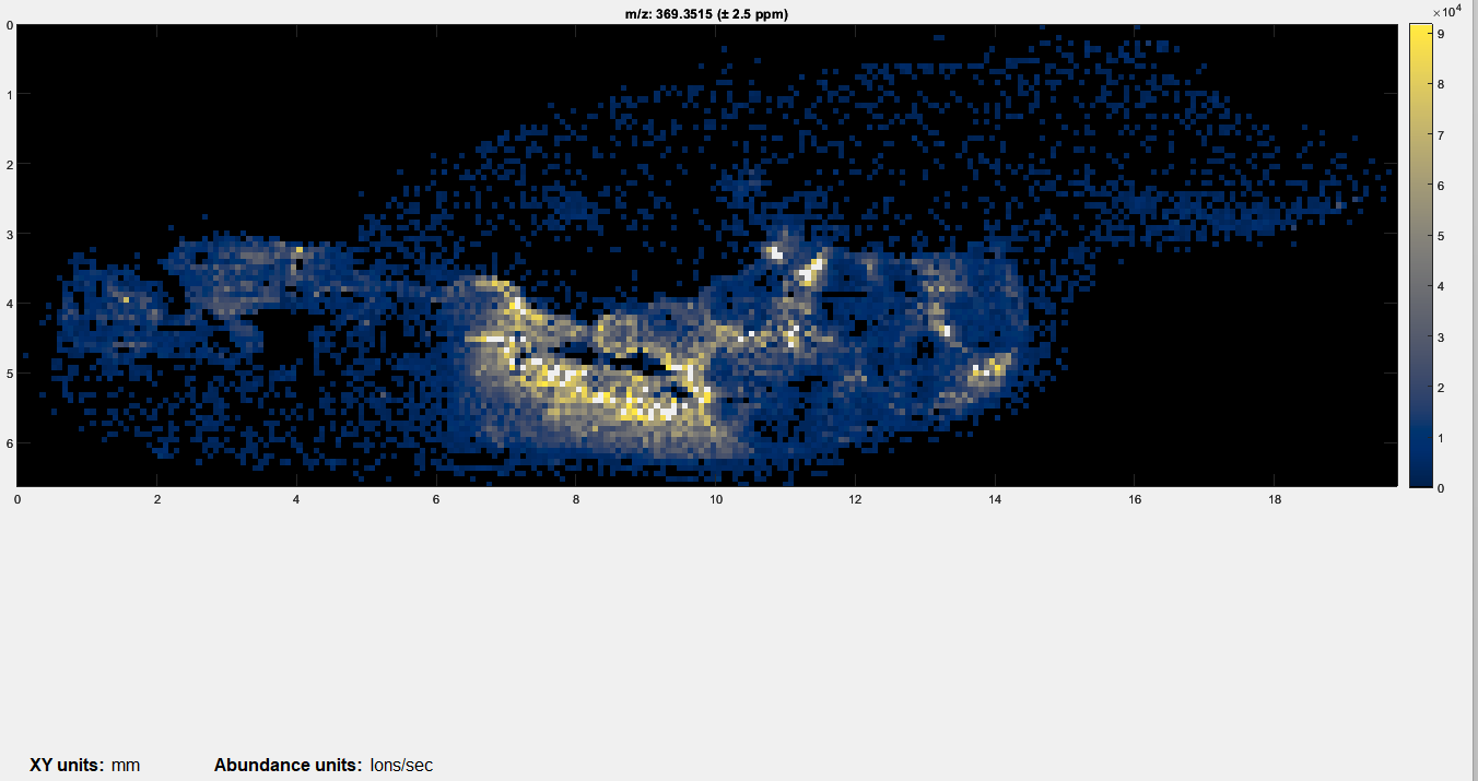
Figure 34: Loading of a mass spectrometry image that was collected with an arbitrary ROI. This is an image of a whole-body zebrafish at 80 micron spatial resolution.
7.1.1.3 The *.mss and *.mim file formats
Once a user has loaded a *.raw file and wishes to save it, it cannot be saved as a Thermo *.raw file (that is a proprietary file format). MSiReader will save this file as a *.mss or *.mim file which then can be directly loaded into MSiReader when further working up a dataset. Please see §3.7 for more information. For example, if a user takes the data shown in Figure 34 and tries to centroid it, MSiReader already knows that it was collected in centroid mode and will automatically chose local maxima for peak picking. If a user applies an abundance threshold of 0.001 (data was loaded with threshold = 0.001 so no change is actually being made), it will prompt the user to save the file as a *.mim file. This file is in the test data folder. Inspection of the file size will reveal the *.mim file is about 1/3 the size of the original *.raw file and loads over 100× faster.
It is important to note that while these data were collected with an ArbROI, the *.mim file format now includes all the information for the data and thus, when loading the *.mim file, the user will not be prompted for a location file.
Once a data file of any type (MSI or BioPharma mode) has been loaded into MSiReader, the user is given the option to save the active session in a binary *.mss or *.mim file format for later use. All data, settings and processing (including colormap and slider positions) will be saved. The session file (*.mss) and the *.mim format also have the advantage of loading up to 10 times faster than the original file, depending on the original format.
When the dialogue box shows up to save the file that is loaded into memory via the main menu (Home/Save session) or the main toolbar icon, the user can select *.mss or *.mim. Here are the details of what will be saved.
If a *.mss file is selected (default), then all the GUI parameters/configs are saved, alongside the data.
If a *.mim file is selected, then on the loaded data is saved, without the GUI parameters/configs.
For both of these file formats, the user can save a loaded dataset without making any modifications to them.
If you wish to save imzML-modified data as a *.mim, a user can now do this.
If the original data came from a single imzML file, then the *.imzML output is default but users can also select *.mim.
If the original data came from multiple files or not from an imzML, then only *.mim output is selectable.
7.2 The MSiReader Main Graphical User Interface (GUI) for MSI Mode
A video tutorial on navigating the main GUI of MSiReader for MSI mode can be found HERE. Note this is an overview of the entire GUI for MSI mode – some of the functions were already described in the user manual.
The main GUI in MSiReader MSI Mode contains 6 panes and includes: 1) MSi Data Attributes; 2) Post-Processing; 3) MS Navigation; 4) Heatmap Mode; 5) Heatmap Appearance; and 6) Colormap. Collectively, these serve as a simple and effective interface to efficiently begin to look at your MSI data with a large heatmap display on the right. Below, each of these panes will be discussed. Please note that when you load MSiReader for a given session, only the MSi Data Attributes pane is shown until a data file is loaded. The overarching GUI with menus, sub-menus, and context menus were discussed in §4 and the description and function of the MSiReaderPrefs.INI were presented in §5. In this section, details will be provided to guide you through the process.
Recall that you should adjust your font sizes to match your display resolution as described in §4.2 using the “A” ICONS in the taskbar for an improved user experience. This can also be done by clicking on the “Visualization” tab and going down and clicking on “Increase font size” or “Decrease font size” repeatedly until the GUI is appropriated sized for your display. You can also set this in the preferences .INI file (§5) default value = 9.
7.2.1 MSi Data Attributes Pane
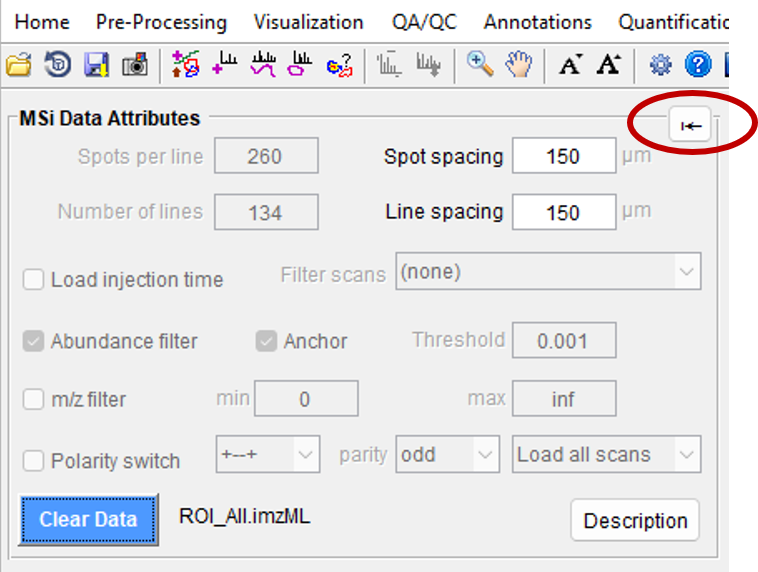
Figure 35: The MSi Data Attributes pane displays the choices that you have set as a default in the MSiReaderPrefs.INI file as well as some values that were imported from the imzML file.
Figure 26 shows the MSi Data Attributes Pane; when you first load MSiReader for a session, this is the only pane that is displayed until a file is loaded. However, prior to loading a specific data set, you can still make changes to these default checkboxes and values. For example, if you used an Arbitrary ROI to collect your data and you have a
location file, you can use the pull-down menus in Filter scans to select “using ROI location file” prior to loading your data.
7.2.1.1 Characteristics of the MSI data
The spots per line, number of lines, spot spacing and line spacing are initially set to the default values in the MSiReaderPrefs.INI file (§5). Spots per Line and Number of Lines entries will be filled in automatically when you load a file unless the mzXML format (single file, multiple files or an entire folder) is selected. The Spot Spacing and Line Spacing fields, relating to the horizontal and vertical spacing, respectively, are loaded automatically from imzML and IMG format files and will affect the dimensions and aspect ratio of the heatmap plots. The Spot Spacing and Line Spacing fields can be changed at any time after the file has been loaded by typing new values into their edit boxes; these manually entered dimensions will be applied immediately. After the file is read, these values can also be modified to change the heatmap plot X and Y axis scaling and the aspect ratio. If set to a negative value the corresponding axis direction is reversed, that is, the heatmap is flipped left to right or turned upside down, respectively. If a value of zero is entered, one unit per pixel scaling is used. Default values can be given in the preferences .INI file in §5.
7.2.1.2 Injection time scaling
Heatmap abundance can be loaded and subsequently scaled by injection time with a checkbox in the MSi Data Attributes pane “Load injection time”. Injection times will either be read from the data file directly or, if not found in the file, the user will be prompted to enter a value during the load process. When the load injection time box is checked, the injection time is read into (or an injection time is manually entered in the dialog box). All of the scans in an image do not have to have the same injection time. For example, an imzML file that is a “stitched” composite of multiple data sets or a folder of imzML or mzXML files. How to use the injection time values will be discussed in §6.2.2.
7.2.1.3 Filtering data
Data sets can be filtered during loading in a number of ways including 1) using an ROI location file (§2.4.3) or a bespoke scan pattern; 2) abundance threshold (§2.4.4); 3) m/z range; and 4) polarity switching. Abundance filtering is the most commonly used but each one of these filtering approaches will be described here individually; some can be carried out simultaneously (e.g., abundance threshold and m/z range) while others are mutually exclusive (e.g., ROI location and bespoke scan pattern). Using an ROI location file when loading data was described in §3.1 and setting an abundance threshold (including the meaning of the anchor checkbox) was described in §2.4.4 and thus, these will not be discussed here.
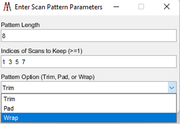
Figure 36: Bespoke scan filter dialog box.
Unwanted scans that follow a regular pattern can be filtered from a data set as it is read with a bespoke scan filter by selecting “using bespoke scan pattern” in the pull-down menu to the right of filter scans. When the load button is clicked the user will be prompted with the dialog shown in Error! Reference source not found. to describe the scan pattern. The pattern specifies the scans to keep from each pattern replication across rows of the image. If the pattern length is not an integer multiple of the number of columns in the image, the last pattern replicate can be trimmed and the pattern will start again on the next row (Trim), rows of the image can be padded with empty scans to fulfill the pattern (Pad), or the pattern can be wrapped around to the next row (Wrap).
While the file is being loaded scans that are filtered from the image are set to empty. For the parameters shown in Figure 26 the odd numbered scans in each row would be read and saved while the even numbered scans would be skipped. After loading is finished, rows and columns that are completely empty will be removed from the image if the preferences INI file variable SqueezeROIEmptyScans is true (§5). Only those rows and columns outside of a bounding box around the non-empty scans are removed if the variable SqueezeROIBorderScansOnly is also true (§5).
m/z range filtering can be carried out for all file formats except *.mss; the scans are filtered by m/z value as they are read. As shown in Figure 26, one can check the m/z filter which will allow the user to set the minimum and maximum values allowed which are zero and infinity, respectively. Data pairs (m/z, abundance) outside of this range will not be saved in the loaded image. The default values for the filter (0 and infinity) can be changed in the INI preferences file (§5). This filtering can be done to break a large file into several smaller ones or perhaps, a user collected 100 images from m/z = 200 to m/z = 2500 and upon inspection of all the data, it is observed that there are no analyte peaks between m/z 1000 and 2500. In either scenario, m/z range filtering will reduce the demand for physical memory.
Data collected natively using polarity switching can be filtered in MSiReader. MSiReader supports analysis of data sets with mixed polarity scans in two ways: polarity filtering and polarity switching. Options for filtering and switching are accessed by right-clicking on the file type pull-down menu in the MSi Data Attributes pane (Figure 26) before a file is read. Polarity filtering and switching are only implemented for the imzML file, mzXML file, imzML folder and mzXML folder data type selections. Also note that polarity information for all scans must be stored in the data set for this feature to be meaningful.
Any data set that contains both positive and negative scans can be filtered by polarity as it is read, retaining only the positive (+) image, the negative (-) image or both (load all scans). The distribution of polarity is arbitrary and an empty scan will be inserted in the image in place of each filtered-out scan. The type of polarity filter is selected before the file is read from the context menu to conserve memory. The default is to load all scans.
In the case where all scans are kept, the MSiSpectrum (§7.6.6) and MSiPeakfinder (§7.7.1) tools have a button to use the positive scans, negative scans or all scans for processing selected ROI(s) if there were both (+) and (-) polarity scans in the data set.
MSiReader supports files that contain four polarity patterns replicated across the rows of the image matrix: [+ - - +], [- + + -], [+ -] and [- +] along with two scan retention options: keep odd and keep even. These choices are accessed by the pull-down menu which is activated if the Polarity switch checkbox is selected. Polarity switching options are selected before the data set is loaded. The defaults are the [+ - - +] pattern and the keep odd option. This can be changed in the preferences INI file (§5).
For the 4-tuple patterns [+ - - +] and [- + + -] either the odd (1,3) or the even (2,4) scans are equilibrium scans with no advancement of the sample raster stage and these scans are not loaded. Since the equilibrium scans are all in the same column of each raster scan line, that column can be “squeezed out” of the resulting image. The other scans, (2,4) and (1,3) respectively, are loaded and MSiReader will then have a positive image and a negative image interleaved by column. As with polarity filtering, the MSiSpectrum (§7.6.6) and MSi Peakfinder (§7.7.1) tools have a button group to use the positive image, negative image or both for processing selected ROI(s). The polarity filter can be used in conjunction with equilibrium scan switching so that only the positive or the negative image is loaded and the unwanted columns are eliminated from the image. For the 2-tuple patterns [+-] and [-+] the keep odd or keep even options are used to specify which image polarity to load (positive or negative) and the polarity filter is disabled (i.e., set to all scans).
If polarity switching is enabled, the first four scans of the file are read and their polarities are compared with the selected pattern. An error is displayed if there is a mismatch. The remainder of the file is not checked for fidelity to the selected pattern. Rows of the data matrix are padded with empty scans, if necessary, so that the number of spots per line is an integer multiple of the selected pattern length (2 or 4). When a scan is selected with the cursor tool  , the polarity and abundance for the scan under the marker is displayed above the heatmap plot as the tool is moved on the screen. Similarly, if an m/z spectrum plot is enabled, the title of the plot includes the polarity of the scan.
If you need more working space for the heatmaps, you can click on the arrow as shown in Figure 26 in the red oval. This will collapse the MSi Attributes pane and the Post Processing pane. Clicking “settings” will recover those two panes.
7.2.2 Post Processing
7.2.2.1 Injection time scaling
If you loaded the injection time when you loaded your data file(s) or manually entered a value via the dialog box, in this pane there is a toggle to either use the injection time (checked) or not use the injection times (unchecked – default value). When using the injection time(s), the ion flux (ions/sec) is multiplied by the scan injection time and the heatmap is updated immediately as well as the abundance units. For example, changing from “ions/sec” (ion flux) to “ions” (total number of ions) if you go from not using ion injection time to using injection time information. If you then uncheck the box for injection time scaling, the abundance data is restored to its previous state by simply dividing by the injection time. The heatmap plot(s) is(are) immediately updated. The default labels (e.g., ions, ions/sec) can be changed in the MSiReaderPrefs.INI file (§5) to match the output of your specific mass spectrometry platform.
7.2.2.2 Peak Normalization
Numerous methods of peak normalization are implemented by MSiReader, including normalization by any arbitrary matrix that has the same number of scans as the loaded data set. In the normalization pane, select the type of normalization using the pull-down list. The default selection is “none”. A label is added after abundance units to reflect that normalization have been carried out. The character strings used for each type of normalization can be changed in the preferences INI file (§5).
Normalization using a single reference peak. The following function is used to normalize the abundance values in the image with the abundance of a specific m/z value. When you select Ref Peaks in the pull-down menu, another box will appear to type in the m/z value of the reference peak (single peak m/z). The tolerance of the reference m/z value is based on the tolerance set in the MS Navigation pane (§6.2.3).

For each spectrum, normalization will only be performed if the abundance of the reference peak is above the user defined threshold, NormCutoff. The normalized abundance is scaled by the NormScale value. Default values for NormCutoff, NormScale and the ReferencePeak can be changed in the preferences INI file as described in §5.
A quick check to make sure proper function is to enter in the same m/z value in Ref Peak data entry field as did for the m/z of interest you entered in the MS Navigation pane. In this instance, you should observe two things: 1) the scale should be one with a heatmap that has a scale of unity and a single color. This is because you have normalized the peak of interest to itself; 2) after the abundance units (below the heatmap), you should see “peak normalization” so you will easily recall that these data were normalized.
Normalization using multiple reference peaks. The end user can also use multiple peaks to normalize the data based on the m/z value (range) of the data. To access this feature, in the main GUI in the post-processing pane, select “Ref Peaks” for normalization and then check “multiple refs” and then click on m/z bounds. A table will appear that has “From m/z”, “To m/z” and “Reference m/z”. For example, if the user has collected data from m/z 200 – 800 and wishes to normalize the data from 200 to 500 and 500 – 800 using different reference m/z values, simply enter in 200 and 500 and the m/z value of reference peak (ref1) in first row and 500 and 800 and the m/z value of the reference peak (ref2) in the second column. Click OK to normalize the data using this approach. In this example, all of the data between m/z = 200 – 500 will be normalized to the abundance of ref1 and all of the data between m/z = 500 – 800 will be normalized to the abundance of ref2.
Normalization using the total ion current (TIC).
When normalization with TIC is selected, every scan is normalized with its total ion current value. If the TIC value for each scan was not provided with the original imaging data file, the user is given the option to use the sum of all abundance values in the spectra as the TIC. TIC normalization will therefore be calculated as follows,

Note 1: For both Ref Peak and TIC normalization, if sum of window or mean of window is selected instead of max of window, Sum or Mean is used instead of Max in the numerator and denominator of Equation (2) and in the numerator of Equation (3).
Normalization using a local total ion current (local TIC).
In the pull-down menu, select local TIC and cutoff and scale will show up (default values are 1) and TIC Bounds. Click on TIC Bounds and a dialog box will pop up. Enter in the bounds for the local TIC (default values are 200 600 1000) which means that a local TIC from < 200, 200-600, 600-1000 and > 1000 will be calculated. More local TIC ranges can be input into the dialog box to define more local TIC regions. For example, 200 400 600 800 1000 will generate 4 local TIC ranges that will be used for normalization.
The m/z intervals are defined by their boundaries with the LocalTICNormBoundaries variable in the preferences INI file (§5). The global m/z range of the data set defines the lowest and highest m/z ranges. For example, setting LocalTICNormBoundaries to “200 600 1000” defines four local TIC intervals:
m/z < 200, 200 >= m/z < 600, 600 >= m/z < 1000, and m/z >= 1000.
If the user wishes to change the local TIC intervals after starting MSiReader, select TIC bounds to enter new values. Local TIC data is immediately calculated for the new intervals if a data set is currently loaded. The smallest value that can be entered is zero and the largest is Inf. The m/z values are sorted and duplicates are removed.
To obtain heatmaps of the TIC (and local TIC’s if selected) go under visualization menu and then select TIC; TIC and local TIC plots are displayed for any m/z intervals that are not empty along with the global TIC plot. Note that the TIC values read from an imzML file are not necessarily the same as the sum of abundances for each scan. Thus, the sum of the local TIC over all m/z ranges may not be equal to the global TIC.
Normalizing to the maximum abundance. First the windowing options are applied. That is, the Sum, Mean or Max within the m/z window is found for each scan. Those values are divided by their maximum and the result is multiplied by the NormScale value. The maximum heatmap abundance will be NormScale and the minimum will most likely be zero.
Normalizing to the mean abundance. First the windowing options are applied. That is, the Sum, Mean or Max within the m/z window is found for each scan. Those values are divided by their average and the result is multiplied by the NormScale value.
Normalizing to the median abundance. First the windowing options are applied. That is, the Sum, Mean or Max within the m/z window is found for each scan. Those values are divided by their median and the result is multiplied by the NormScale value. Note that a non-empty scan can have zero abundance after median normalization.
Normalizing to the midpoint of the abundance range. First the windowing options are applied. That is, the Sum, Mean or Max within the m/z window is found for each scan. Those values are divided by their midpoint and the result is multiplied by the NormScale value.
Normalizing with a custom heatmap. Custom heatmaps are typically created by combining or post processing abundance data in Excel. See §7.2.6 below for more details about custom maps. Normalization with custom heatmaps enables the user to apply an arbitrary normalization scheme to a data set. As an example, if you want to normalize imaging data to the sum of the abundance of other analytes (e.g., drugs and metabolites) you can use the image summation feature to create a file suitable for loading as a custom heatmap. See §7.2.6 for more details. In this case, the exported data is a single column of values in a text (.txt extension) file. You can also create Excel files containing the results of combining exported image data in other ways. When selecting an Excel worksheet as a custom heatmap the data selected must have the same number of values as the number of scans in the loaded data set but they do not have to be arranged into the same number of columns and rows. The custom normalization data can also be a single value. It will be expanded to a matrix with dimensions that match the loaded data set.
7.2.3 MS Navigation
The MS Navigation is shown in Figure 27 to navigate your data using different analytical figures of merit.
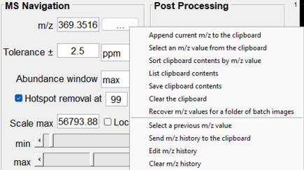
Figure 37: The MS Navigation Pane which includes data entry fields of m/z, tolerance, abundance determination, hotspot removal, scale max. scale lock and min and max slider bars to scale the heatmap. If you right click on the ”…” next to the m/z field, there is a context sensitive menu that provides options for moving m/z values to the clipboard as shown.
Once an image is loaded in MSiReader, the user can manually enter va;ues in the m/z field. Below are descriptions of the options available in the MS Navigation pane.
7.2.3.1 m/z
Location on the m/z scale where the m/z window is centered. Note that it is possible to append m/z values to the clipboard by accessing the right-click context menu of the m/z edit box. A peak list can therefore be easily generated while navigating the data set and then used with the correlation and batch processing tools (§7.6.5) or pasted in Excel for later use. The right-click context menu for the m/z edit box (see Figure 28), contains items to access clipboard and history features that aid image navigation and make it easier to build lists of m/z values for batch processing and for saving in a document or spreadsheet.
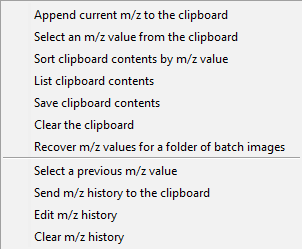
Figure 38: Context menu for clipboard and m/z history functions.
Whenever the heatmap plot is updated the m/z value is automatically added to the history. The clipboard is the windows system clipboard, so it is not necessarily empty when MSiReader is launched and anything added to it is available after exiting MSiReader. For example, the m/z values can be pasted into a column of an Excel worksheet while MSiReader is active or after exiting. Both the clipboard and the history are preserved when the loaded data set is cleared and new data is loaded. The m/z history is lost when the MSiReader session terminates.
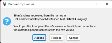
Figure 39: m/z recovery clipboard dialog.
Selecting the last item in the top section of the context menu, Recover m/z values for a folder of batch images, will prompt the user to select a folder and then attempt to build an m/z list from the names of the graphics files (bmp, emf, eps, jpg, pdf, png, tif, or fig) in the folder. For example, MSiReader’s correlation and batch processing tools (§7.6.5) and figure export (§7.6.6) tools create file names containing mmm_zzzzz.ext, where mmm.zzzzz is an m/z value and ext is one of the graphics file type extensions. This can be particularly useful when the contents of a folder have changed. For example, curating a folder of putative peaks with a viewing application. If any m/z values are recovered from the file names in the folder the user is prompted to either append them to the clipboard or replace the contents of the clipboard with the list as shown in Figure 29.
7.2.3.2 Tolerance
Size of the window considered for the calculation of the abundance of the m/z peaks. The user can choose to have a fixed m/z window in Thomson (Th) or a relative window in parts-per-million (ppm). Note that the m/z window size units selected will also be used by the MSiPeakfinder tool (§7.7.1).
7.2.3.3 Abundance
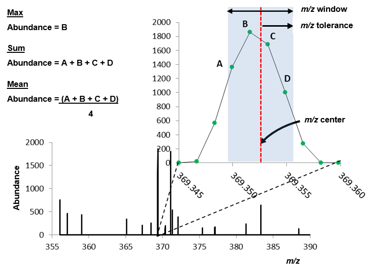
Figure 40: Definition of m/z window, m/z tolerance, m/z center and the three methods used by MSiReader to report ion abundance (max, sum, and mean).
MSiReader offers three different methods to map abundance to a color displayed on the heatmap: 1) the maximum abundance value in the m/z window (window max); 2) the sum of the abundance values in the m/z window (window sum); or 3) the mean of the abundance values in the m/z window (window sum). The meaning of these three options is shown in Figure 30. Note that the reported abundance and m/z value are not necessarily the values at the center of the window.
7.2.3.4 Hotspot Removal Tool
The appearance of a heatmap image is occasionally dominated by a small number of pixels whose abundance is much greater than the rest of the image. To apply the hotspot removal tool, simply check the box and then set the percentile level; the default is to have it enabled with a percentile of 99%. Enabling hotspot removal dramatically improves the appearance of the heatmap image by saturating pixels above the selected percentile level. This is achieved by automatically adjusting the max color scale slider bar to the abundance value corresponding to the hotspot percentile level. This algorithm is identical to the one used by METASPACE11.
7.2.3.5 Min/max slider bars
Values for the minimum and the maximum abundance values represented by the color scale. All scans with an abundance outside of this range will be displayed with the most and least color intensities.
7.2.3.6 Scale Max
The default value for the abundance max slider bar is the maximum abundance of all the scans. For finer adjustment of the color abundance scale, simply change this value. There is also a Lock colorscale checkbox context menu item on the scale override field. This is useful for comparing images visually by forcing identical color bar scales regardless of the maximum abundance value. It applies to normalized data set in the MS Navigation pane as well as batch processing (§7.6.5).
Note: all default values can be modified in the preferences INI file (§5).
7.2.4 Heatmap Mode
The user can choose to generate heatmaps using the MSi data or to load custom abundance data from a file (Excel or text). These 2 modes are described below.
7.2.4.1 MSi File Data
When this mode is selected, heatmaps are generated using the data from the MSi file. In this mode, all data processing and toolbar tools are enabled. This is the default mode of operation. This can be selected under Visualization > Heatmap Normalization > Use Loaded File Data. In this case, the user can select different normalization in the Post-Processing pane of the main GUI in MSI and BioPharma Mode.
7.2.4.2 Custom Heatmap
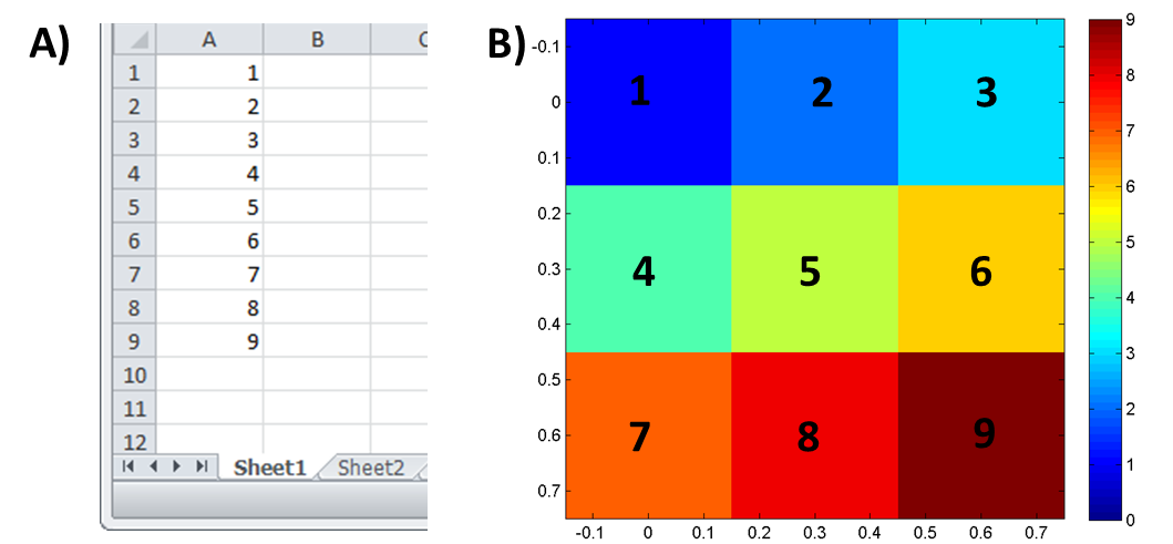
Figure 41: Simple example of custom heatmap loaded for a 3×3 image where abundance increases from 1 to 9. A) Excel spreadsheet containing the abundance values and B) resulting heatmap.
When this mode is enabled, the user can use custom data to generate a heatmap. Data can be loaded from an Excel spreadsheet or a *.txt file. If the Excel file contains multiple worksheets the user is prompted to select one of them. MSiReader expects N abundance values where N is the number of scans in the image (number of rows times number of columns) or a single value. The first value is the scan in the top left corner and the last value is the abundance at the lower right corner (every line from left to right) as shown in Error! Reference source not found.. This input format (order of abundance data point) was chosen since it is the same format as the output format for the abundance extraction tool. If the input worksheet (or text file) contains a matrix with the correct number of elements, then it will be used as the custom heatmap. If not, then if the first column contains N values it will be used. The user can therefore extract data points using the abundance extraction tool (after selecting all scans in the image as a ROI) and perform any processing of that data in Excel before reloading the results as a custom abundance heatmap. The MSiSlicer tool can also export a 2D cross-section of data and the entire abundance heatmap (§7.4.6). The format of this exported data is appropriate for input as a custom abundance heatmap.
For example, if a user would like to make a custom normalization by summing up the abundance of specific m/z values in the data, here are the steps.
Under the visualization menu, select “summed m/z abundance”. Enter in the m/z values that will be summed. It will automatically display a heatmap of the summed abundance and then prompt the end-user to enter in a *.txt filename for this custom heatmap. Save this file.
Next, under Visualization > Heatmap Normalization, select “use custom abundance data”. Because this custom abundance data was created with the data, it will have the same ROI dimensions. It will prompt the user to load the *.txt file that was just created. Notice then when it is applied, it automatically updates the heatmap. If a user wants to undo the application of the custom heatmap, simply return to the Visualization > Heatmap Normalization and select “use loaded file data”.
Finally, in creating the abundance data, another *.txt file was also automatically created with the same filename with added extension _mzlist so the user knows which m/z values were summed for the custom heatmap.
7.2.5 Heatmap Appearance
7.2.5.1 Interpolation
The pixel interpolation scheme can be changed in the Heatmap Appearance menu. Three types of interpolation are available (linear, spline and cubic) and each type can be applied up to the 5th order. For each type, selecting zero order will revert to non-interpolated data (i.e., none). Applying an interpolation scheme does not change the stored data since it is only an image processing step. Default interpolation is linear of order zero (i.e., no interpolation). This can be modified in the preferences INI file (§5). When an ROI drawing tool is enabled, the interpolation order is temporarily changed to zero so that scan boundaries are clearly visible.
7.2.5.2 Sequential Paired Covariance (SPC)
A sequential paired covariance (SPC) visualization feature has been added to the Heatmap Appearance panel. SPC reduces the effect of variable noise peaks in an image. It is a visualization tool and does not modify the underlying spectral data.
SPC is a way of visualizing data with large dynamic range as well as defining changes (e.g., tumor margin) which may otherwise not be apparent. This algorithm was recently published for mass spectrometry imaging12 and was based on previous work with liquid separations coupled to mass spectrometry13,14. First, the user selects the checkbox and that allows the user to then choose the SPC Options. The first is the threshold with a default value of 1. The second is the log base you wish to use. The third entry is the filter function which can be product, sum, median or midpoint. Given that the default for the heatmap update is checked, when you chose these different options, using the m/z value entered in the MS Navigation pane, you will observe the SPC heatmap.
SPC is calculated for each pixel in a heatmap as the logarithm of the product of that pixel’s abundance with the abundance of the adjacent pixels. The corner pixels have only three neighbors, the other pixels on the first and last row and column have five neighbors, and all interior pixels in the image have eight neighbors. SPC is enabled with a checkbox and has three options that are accessed from a context menu on the checkbox label: an abundance threshold, the base of the logarithm, and the filter function. Abundances below the threshold are excluded from the calculation and the default threshold is 1. This prevents zero or very low abundance values from propagating in the image. The default logarithm base is e (2.7183). Setting the base to any value less than or equal to 1 disables the logarithm step after the dot product is formed. The filter function default value is product. Three other choices are sum, median and midpoint.
The colorscale slider bars and colorscale override can be used to reduce the upper and lower abundance assigned to the most and least intense colors respectively. Increasing the minimum value can be helpful for reducing the influence of the background on the image.
SPC can be used with any of the abundance treatments (window mean, window max, window sum), normalization options, hotspot removal, interpolation, and log color scales. If enabled when the MSiCorrelation and batch processing tool (§7.6.5) is launched it with be applied to batch images as they are generated. Three variables were added to preferences INI (§5) file to set the default values for the SPC options.
Variable Value
SPCEnable false
SPCThreshold 1
SPCLogbase 2.7183
SPCFilter product
7.2.6 Colormap
The default colormap is cividisblack which is color vision deficiency compliant3,4 and presents a heatmap that is representative of the data. It is a perceptually linear colormap instead of a “rainbow” style colormap like the previous default, jet, which has long been considered misleading for the presentation of scientific data3, especially when converted to grayscale and printed.
The scaling is a simple a way to better display large dynamic range data in the heatmap when you have an analyte that varies over orders of magnitude in abundance within your image. The user can choose from linear, log base 10, log base 2, and log base e. If you wish to “flip” which color is most abundant and which is least abundant, check the “flip” checkbox.
7.3 Pre-Processing Menu
7.3.1 Mass Correction
A video tutorial on how to use the mass correction tool can be found HERE.
You can check your MSI data quality using the QA/QC tools described in §7.5. In the event that upon plotting out your data using the mass measurement accuracy heatmap and/or histogram tool is not within the specification of your instrument, you can use this tool to do a single-point mass correction (this is not a full mass re-calibration routine).
The MSiReader external mass correction tool can be used to improve the MMA for a given data set. The calibrated results are displayed as a heatmap showing the ppm shift for each pixel in the image and are optionally saved into an Excel workbook. The loaded data can also be updated in MSiReader with the new m/z values for each scan. Finally, the corrected data may be saved as a new .imzML and .ibd file for permanent storage. Alternatively, the user can save the mass corrected data as a *.mim file which is about 1/3 the file size and loads significantly faster.
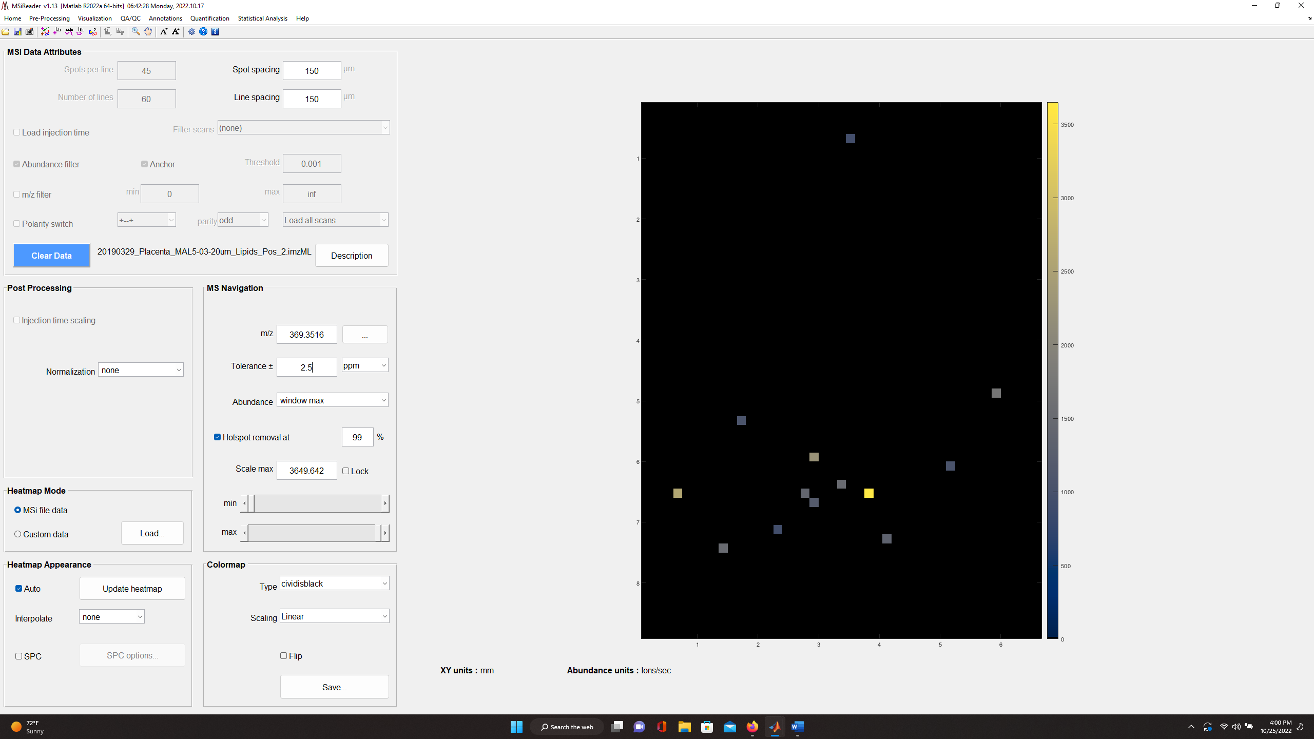
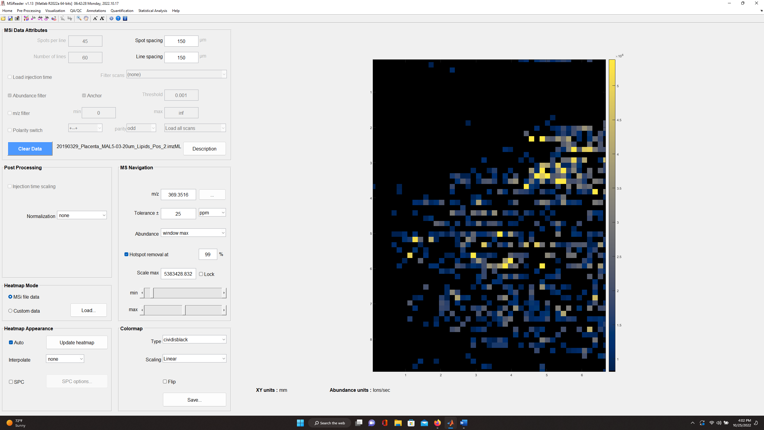
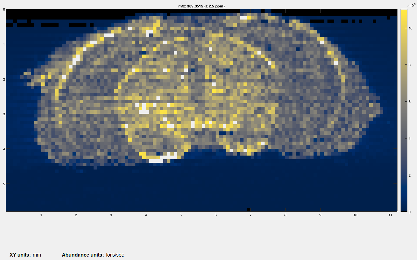
Figure 42: Heatmap of cholesterol in mouse placenta with ± 2.5 ppm (top)
and ± 25 ppm (bottom) tolerance windows. This indicates that the mass measurement accuracy is not within specification and thus, a mass correction of the data is required.
For example, for the mouse placenta tissue in Figure 42 (top) cholesterol (m/z 369.3516) with a tolerance of ± 2.5 ppm should be highly abundant across the sample and in fact it is when the tolerance window is increased to ± 25 ppm as shown in Figure 42 (bottom).
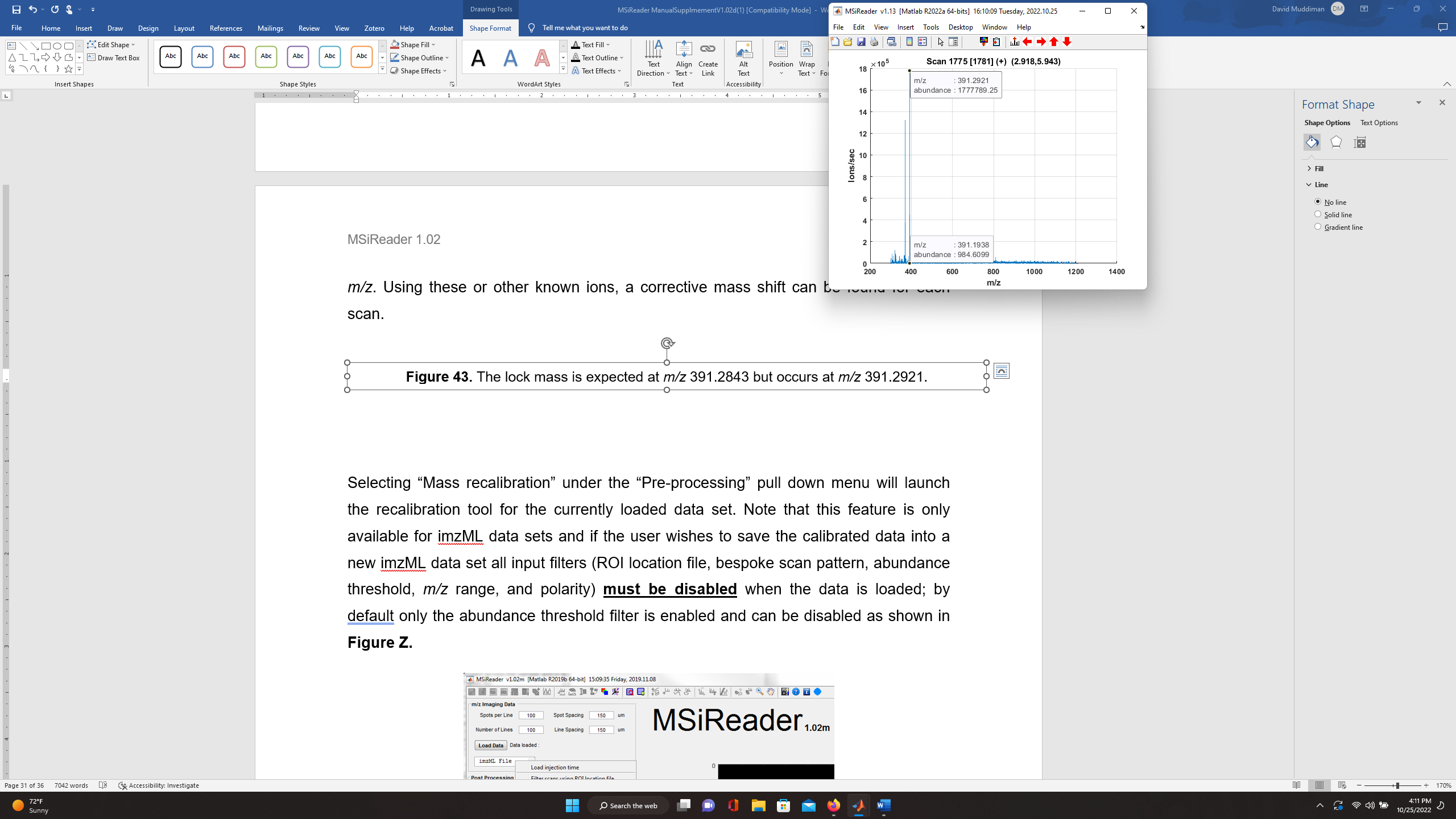
Figure 43: The lock mass is expected at m/z 391.2843 but occurs at m/z 391.2921.
It is also apparent from the mass spectrum shown in Figure 43 that a lock mass (m/ztheo 391.2843) typically used on this instrument platform also has poor MMA (19.934 ppm; m/zobs = 391.2921). Using these or other known ions, a mass correction can be determined for each scan and applied.
Selecting “Mass correction” under the “Pre-processing” pull down menu will launch the single-point mass correction tool for the currently loaded data set. Note that this feature is only available for imzML data sets and if the user wishes to save the calibrated data into a new imzML data set all input filters (ROI location file, bespoke scan pattern, m/z range, and polarity) must be disabled when the data is loaded; by default, only the abundance threshold filter is enabled which is allowable.
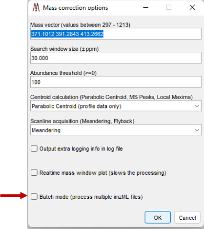
Figure 44: External mass calibration user options dialog box. If the user inputs values that are not allowed, when OK is selected, the dialog box will remain present on the screen until the user fixes the error. For example, notice that the input for mass vector for the calibrant ions, an m/z range is noted that is allowed for the loaded dataset.
After selecting the “Mass correction” tool, the dialog box shown in Figure 44 is displayed. The default values for these settings can be changed in the preferences INI file (§5). Any number of m/z values can be entered and the search window ppm value can be specified as a vector with a value for each m/z. For each scan, the most abundant peak within the mass window for each calibration value will be found and the most abundant of those entered will be used for calibration. Peaks are found using one of the three centroid algorithms implemented by MSiReader. If you are mass correcting profile data, you must use either Parabolic Centroid OR MS Peaks. If the user is mass correcting centroided data, one must use Local Maxima. The scanline acquisition parameter will default to the value read from the metadata by MSiReader. However, it should be noted that this is not a required parameter in the file so the value in the dialog should be confirmed by the user or the results cannot be correctly saved to a new imzML dataset. The batch mode (red arrow in Figure 44) for mass correction is discussed below at the end of this section.
The real-time mass window plot option shows the tolerance window around each calibration mass as the scans are processed in the same plot as shown in Figure 45. The plot can be closed at any time and it will not be recreated. Note that the real-time plot degrades performance substantially.
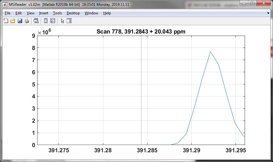
Figure 45: Real-time plot is updated while searching calibrant m/z values.
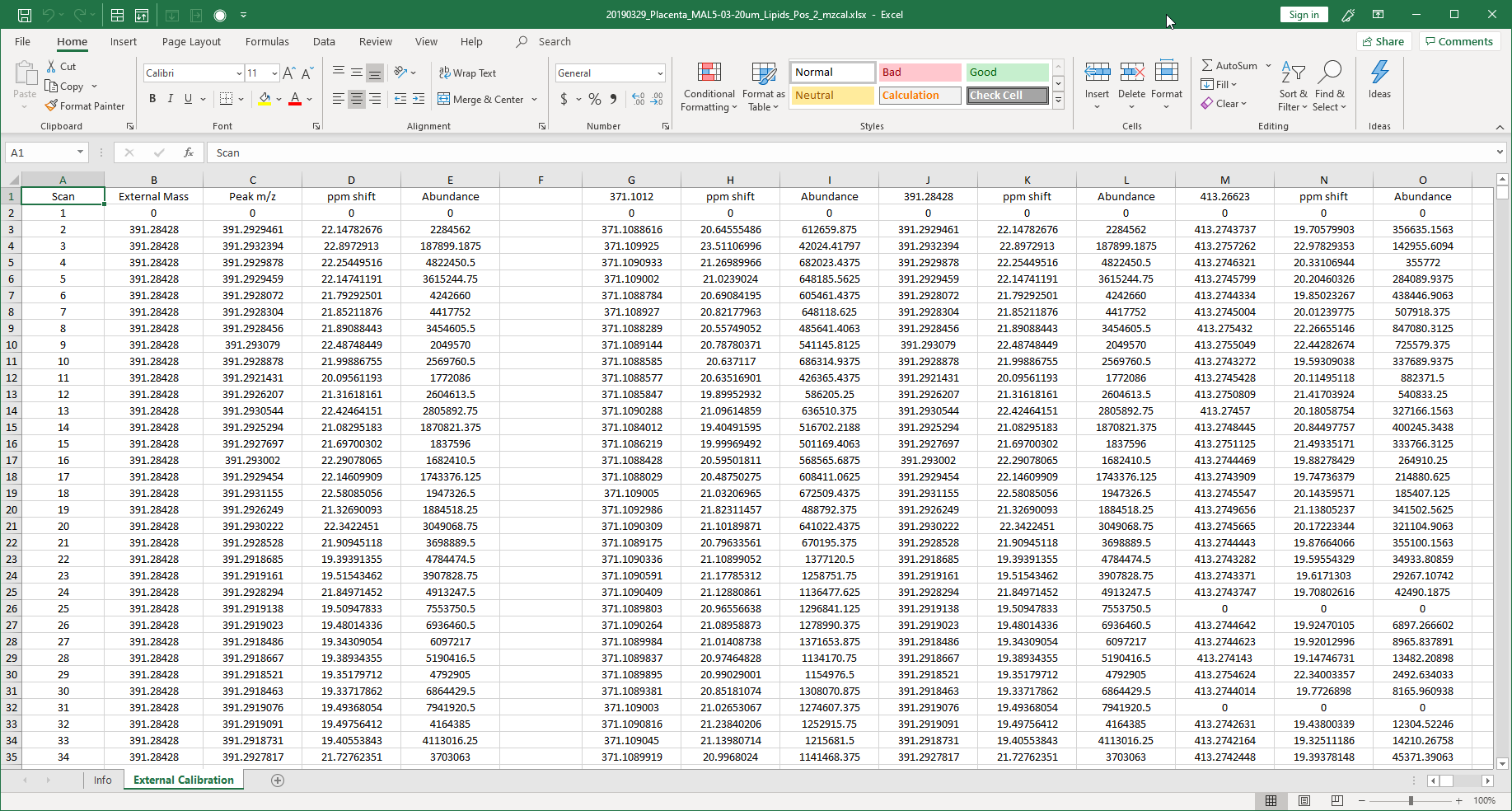
Figure 46: The observed m/z, ppm shift and ion abundance for each of the external calibration masses that were entered into the dialog box (Figure 45).
Upon completion the user is asked to select a place to save a report summarizing the results in an Excel workbook. An example is shown in Figure 46. The report includes the m/z, abundance and ppm shift for all masses and tolerance windows. The ppm shift heatmap shown in Figure 47 summarizes the results graphically. This is optional and does not have to be saved.
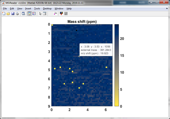
Figure 47: External mass calibration ppm shift heatmap. The data cursor shows the selected peak m/z and MMA (ppm) for the queried scan.
The mass shift plot toolbar icons allow the user to see a before-and-after spectrum plot for the scan under the cursor  (Figure 48), update the m/z values in MSiReader
  (Figure 49), and save the results into a new imzML data file or a *.mim file format.
When saving the calibration results into a new imzML data set, the .imzML file is copied unchanged and the .ibd file copied and then new m/z vectors are written for each scan. Note that if one or more ROIs are active when the external tool is launched, the user will be prompted to select either ROI scans or all scans. Only the selected scans are processed, plotted and modified.
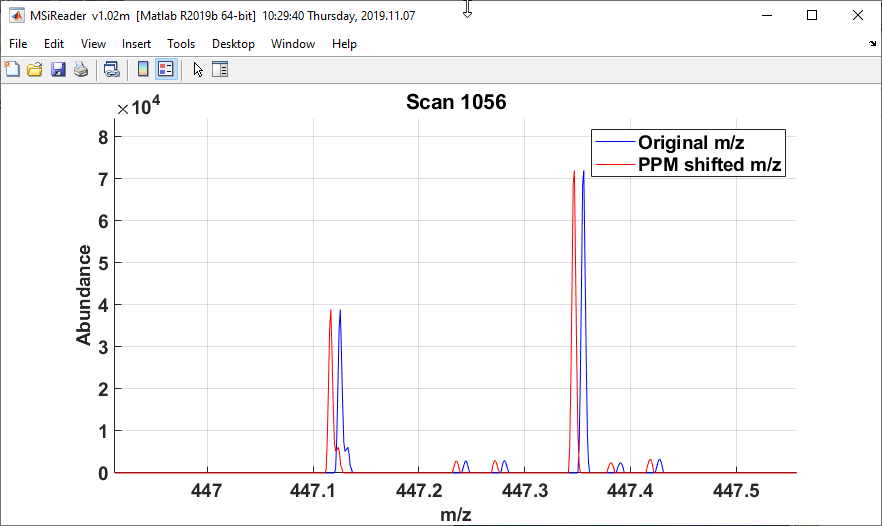
Figure 48: The original (blue) and m/z corrected red) spectrum for scan 1056.
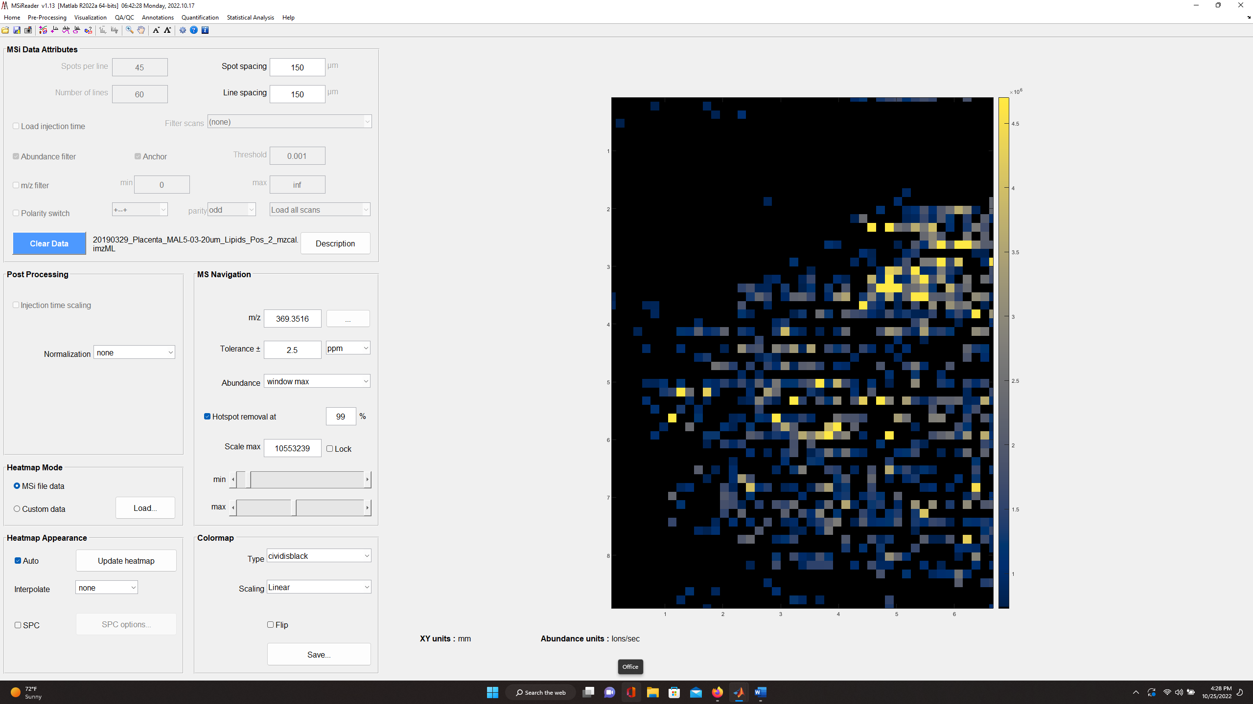
Figure 49: Heatmap for cholesterol with +/- 2.5 ppm tolerance after loading the mass corrected data.
The batch mode for mass correction is to allow the end-user to carry out a single-point mass correction on multiple imzML files without having to load them, save the calibrated data and then save the new imzML file. This function can be accessed in two different ways. The batch mode is not yet functional for *.raw files.
First, you can load an imzML file as before and then launch the mass correction tool which will show you dialog box as shown in Figure 44. Make sure the values in this dialog box are suitable for your dataset. Next, check the box that says Batch Mode and then OK. This will open a folder for the user to select one, two or an entire folder of imzML files. After selecting the files and then OPEN, MSiReader will automatically do a single-point mass correction on every imzML file that was selected and then write the corrected data to a new imzML file with an extension to each filename _mzcal. Since this is batch mode processing, the user does not have to load a dataset – the user can access Mass correction as before directly from the Pre-Processing Menu. In this approach, since no data is loaded into memory, the Batch Mode is automatically checked (and cannot be unchecked). After your parameters are set, select OK and then the file explorer will open as before, select which imzML file(s) you want to mass correct and then OPEN. MSiReader will do as before and recalibrate the data and add an _mzcal to each file that was selected for mass correction.
7.3.2 Centroid Data and Peak Exclusion Filter
A video tutorial on centroiding data and peak exclusion filter can be found HERE.
Note: This section is partially repeated from Part I: Getting Started
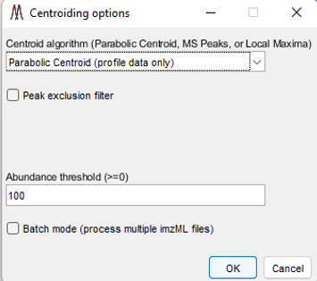
Figure 50: Centroid Data Options Panel in MSiReader
MSiReader can take your profile data and centroid it for you – this will reduce the file size and therefore reduce the amount of RAM required. This feature was added to enable some tools to be used in MSiReader that require centroided data but can also be used to reduce file size to the data in memory or using the batch mode. Under the Main Menu item “Pre-Processing” select “Centroid Data” function as shown in Figure 50. You can select from three different centroid algorithms (if you are using this tool on data that is already centroided, you must choose “Local Maximum” as the Centroid algorithm), set an abundance threshold, turn on or off the peak exclusion filter (peak exclusion can only be carried out using centroided data – in this case, it will centroid your data and then apply the exclusion filter) and set your peak tolerance in this panel. Then select OK. If you check the peak exclusion filter, you will be prompted for a list of m/z values. If the clipboard contains a positive number within the m/z range of the loaded data set you will be asked if you want to use those values as the exclusion list. If it contains other content or you decline you will be prompted to select a .txt or .xlsx file with the m/z values that you wish to exclude. In the case of selecting a .xlsx file with more than one worksheet you will be prompted to select one. For both types of files, the first column of values will be used.
The exclusion list could be background ions that are present in high abundance in every spectrum that will be removed from the spectra and heatmap. They could also be MALDI matrix ions. If the user does not check the peak exclusion filter, it will centroid your data using the other parameters you have selected in the options panel (Figure 50).
Upon centroiding your data in memory, you will be prompted to save a new imzML file in the same folder – MSiReader will add the extension _centroided to the original filename but the user can enter in any filename they choose prior to saving. For batch mode centroiding of data, it will aways add _centroided to each filename automatically and save them in the same folder as the original data. The user can also opt to save these as a *.mim file format.
IMPORTANT: Centroiding data may produce unexpected results if the input file is not an actual mass spectrum but a peak list (preprocessed centroid data). All data preprocessing steps (whether MSiReader or other software) should be validated in your workflow prior to applying them to your data to ensure artefacts are not introduced.
If you check Batch mode and then OK, a file explorer box will open and then you can chose a folder and then select one, several or all .imzML files that the user wants to centroid. This process is carried out in the background. As an example, the .ibd file size for the profile data (in Mass Correction Folder) was ~1.2 GB but after the centroid algorithm was applied, the file size dropped to ~89 MB.
You can simultaneously do abundance thresholding which will further reduce the RAM required (§2.4.4). Moreover, prior to (or after using Scan scrubber tool) centroiding your entire dataset that has been loaded, you can use the ROI selection icon for a polygon and after you select the data of interest, then go to Pre-Processing and then Centroid Data and it will prompt you to select “ROI Scans” or “All Scans”. Once you draw your polygon for the data of interest, if you want the polygon to be a square, right click on the heatmap and select “Make ROI a Rectangle”. You can click on the square and move it around to position it over the ROI of your choice.
There are 3 options to centroiding as shown in Figure 51 which include Local Maxima, Parabolic Centroid and MS Peaks (wavelet transform – not shown). Only use Local Maxima for data for previously centroided data in the case where you wish to apply a threshold and/or peak exclusion filter. This is recommended because Local Maximum, when applied to profile data using most software, will likely compromise your mass measurement accuracy and ion abundance. This is of course the fastest of the three centroiding algorithm; however, be cautious centroiding data using this approach.
.
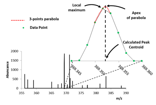
Figure 51: Illustration of centroid algorithms / calculations showing local maximum and parabolic functions.
MS Peaks uses a wavelet transform and filter to find peaks and is similar to the CWT algorithm for peak picking in MSConvert5. This algorithm finds peaks in a noisy signal by smoothing the data using a wavelet transform (Daubechies filter banks), putative peak locations are determined and then post-filtering to reduce over segmented and noisy peaks. This approach to centroiding will likely increase computational time significantly.
These could be background ions that are present in high abundance in every spectrum that will be removed from the spectra and heatmap. If you set peak exclusion as “false”, it will centroid your data using the other parameters you have selected in the options panel (Figure 50).
Important Note: Once the user has centroided their data in MSiReader, the modified imzML file can only be read by MSiReader due to our proprietary parsing algorithm and padding to reduce file size. Regardless, the .ibh, .imzML and .ibd files must all be present to open the file for analysis.
7.3.3 Scan Scrubber
For a video tutorial on how to use Scan Scrubber, click HERE.
The scan scrubber allows a user to load a file, select a single pixel, line or polygon (using the ROI selection tools) and then remove the data either inside the ROI or outside of the ROI. After this process is carried out, the user can then update the heatmap and save these new data. For example, if a user has a file with a lot of noise in the off-tissue pixels or a very abundant pixel that is skewing downstream statistical analysis, one can select an off-tissue polygon ROI or single pixel ROI and then clear them and then save as a new imzML file or *.mim file. It will prompt the user to enter in a filename; however, MSiReader will automatically add “_scrubout” or “_scrubin” to the end of the original filename.
7.3.4 Ion Classification Tool
In mass spectrometry imaging of tissues, it is important to objectively determine whether an ion is tissue-related (on-tissue) or is a background ion. A tool based on object image analysis was recently reported and is now part of MSiReader.15 Below are the steps in order to use this new tool properly. It is important to note that the published algorithm was modified to significant enhance computational speed; the version in MSiReader v3.12 is over 100 times faster than the published algorithm.
The first step is to create to a list of m/z values from the imaging data prior to running the ICT algorithm. This can be done using two different methods:
Method 1 uses the polygon ROI tool to draw an ROI across the entire image. Right click on the image and “select all pixels for the ROI”. Next, under Annotations > Data Export, launch MSiSpectrum. Under “Algorithm for Peak Centroid Calculation” – make the appropriate selection for the data. If the data is already centroided, the end user must select “Local Maxima”. If the data is profile data, the end user must select “Parabolic Centroid” or “MS Peaks”. The user can also apply an abundance filter at this step as well. Next, click “Browse” and enter a filename for these data. This will generate a *.xlsx file that will be used in Step 2.
Method 2 can also be used by exporting the annotation file from METASPACE that can be used in Step 2.
Figure 52: ICT sub-GUI where the list of m/z values (generated by method 1 or 2 above) is selected as well as user-defined variables for the algorithm.
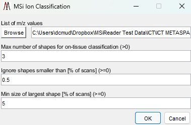 Launch the ICT algorithm which is found under the menu item pre-processing and sub-GUI will be displayed as shown in Figure 52.
The default values for the ICT are based on experience; however, if you are imaging a multi-organ system (e.g., zebrafish), it is normal for a molecular to be distributed in specific organs only and thus, the maximum number of shapes should be increased to allow for that heterogeneity. The higher the value, the more conservative the ICT is to not calling a species a background ion.
Click OK to run ICT. After it is done, it will prompt the user to give a filename for the output Excel file which will have 4 worksheets: 1) unified results: 2) On tissue; 3) Background; 4) mz out of range; and 5) not detected. These are provided so that the end-user can look at the results and perhaps make changes to the variables that go into the ICT specific to their study.
The logic for determining which classification is chosen, is based on object-based image analysis (OBIA) is as follows:
If no shapes are detected, the ion is classified as not detected (essentially low detection frequency);
If the largest shape consists < 5% of MSI scans, the ion is classified as background regardless of the number of detected shapes;
Given an entry for the number of shapes = 3, if 4 or more shapes are detected, the ion is classified as background; if 1-3 shapes are detected, the ion is classified as on-tissue.
This Excel file can then be used to filter the dataset using the peak exclusion filter (§7.3.2) to remove these background ions from the data set and then re-writing a new imzML file. In this case, when the user checks the peak exclusion filter, they will be prompted to choose which worksheet contains the data they wish to exclude. This is an important pre-processing step prior to doing downstream statistical analysis. For example, in DESI and ESI post-ionization methods, removing significant numbers of ambient ions from the data is critical to ensure that an end-user is not, for example, using PCA, separating out a cancer versus healthy tissue sample based on these ambient ions. In MALDI, matrix ions should be removed from the data prior to further processing as these can also drive incorrect conclusions which have nothing to do with disease versus healthy but variability in the MALDI matrix ion signals.
7.4 The Visualization Menu
7.4.1 Abundance Rank
A rank plot is a quick tool to plot m/z spatial distribution as a function of rank in abundance. Using the drop-down menu, choose abundance rank and a dialog box will pop up. If the user selects 1, the m/z value for the most abundant peak (base peak) at
each scan will be plotted on the heatmap. By selecting 2, the m/z distribution of the second most abundant peak will be shown for every scan. Although the usefulness of these plots is limited to higher abundance peaks, it is a quick way to extract some features. An example of this type of plot is shown in Figure 53. Two icons have been added to the rank plot toolbar. Clicking on the 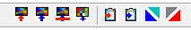 icon updates the MSiReader heatmap with a data cursor m/z value. If there are multiple data cursors the user is prompted to select one. The selected m/z value is also added to the m/z history list when the heatmap is updated. The icon appends all of the data cursor m/z values to the clipboard.
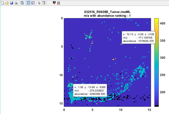
Figure 53: Example of an abundance rank plot. The data cursors show the X,Y location, scan number and m/z values for the most abundant ion in scan 9395 (m/z = 279.2328) and for a widely distributed ion at scan 3128 (m/z = 171.1381).
7.4.2 Total Ion Current (TIC)
The total ion current (TIC) for each scan is plotted in a heatmap by as shown in Figure 54. This is simply a tool to visual the TIC at each pixel across the heatmap.
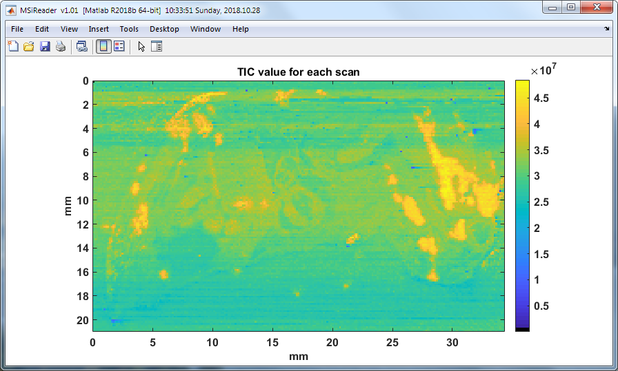
Figure 54: The total ion current for each scan in the image. Notice that in this TIC heatmap there are distinct regions that have higher abundances than other regions. This could be biological in origin based on the structure and or tissue type (e.g., cancerous or healthy) or could be related to the variability of the analytical platform.
7.4.3 Number of analytes
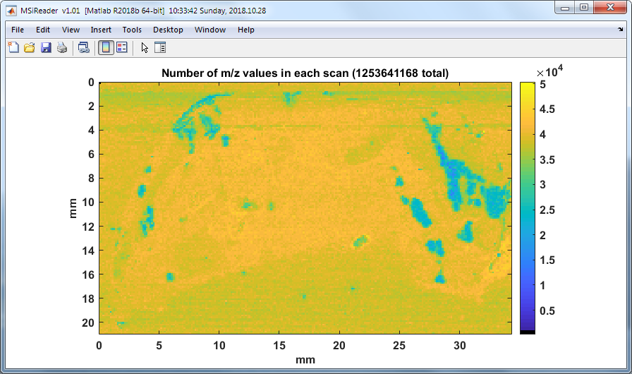
Figure 55: The number of m/z values for each scan.
The density of m/z values (analytes) across an image can quickly be viewed by clicking on “number of analytes” from the drop-down menu under visualization. A heatmap whose color is proportional to the number of m/z values in each scan is plotted in a new figure. An example is shown below in Figure 55.
7.4.4 Summed m/z abundance
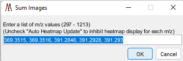
Figure 56: Image summation dialog.
Images for a list of m/z values can be summed by choosing the “summed m/z abundance” in the drop-down menu under visualization. The user is prompted to enter a list of m/z values separated by commas or spaces as shown in Figure 56. The default entry is the most recent five values in the m/z history list.
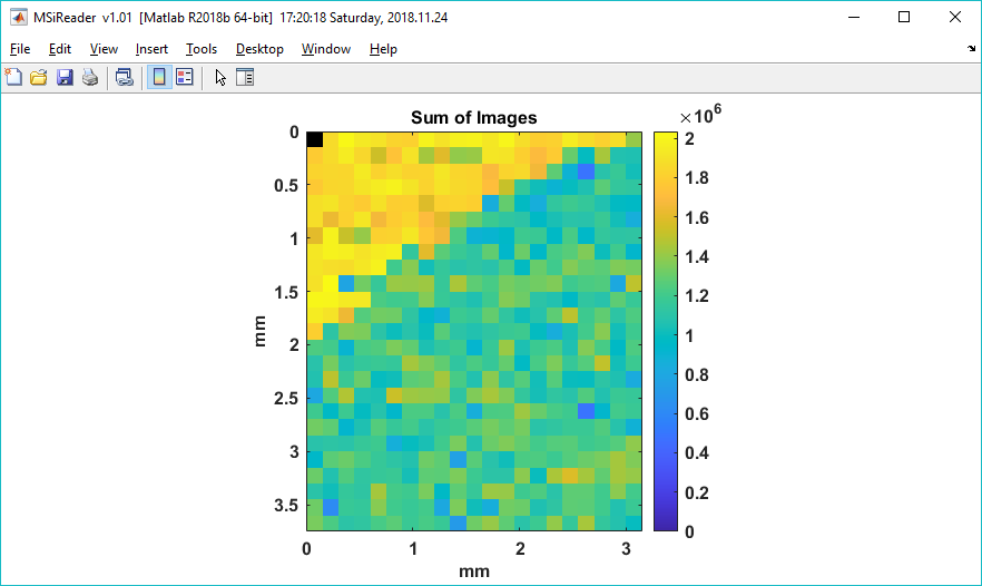
Figure 57: Heatmap of the summation of the user selected m/z values.
A heatmap showing the total ion abundance of the m/z values chosen by the user is exported and an example is shown in Figure 57 and the user is prompted to save the summation matrix into a text file. The text file can be loaded as a custom heatmap (§7.2.4) and used to normalize the loaded data set (§7.2.5). A second text file is also saved containing the m/z list. Note that the summation is for the normalized and windowed m/z as displayed using the criteria in the MS Navigation pane, not the abundances of the RAW scan data.
7.4.5 Spectra above and below a threshold
The heatmap of the distribution of scans above and below a threshold for the current m/z chosen in the MS Navigation pane is carried out using this tool. The user is prompted to enter an abundance threshold and an abundance tolerance with the dialog box shown in Figure 58. The default values are the median abundance and 1/100th of that value for the abundance tolerance for the current m/z. A plot similar to the one in Figure 59 is displayed showing the distribution of scans whose abundance is within the tolerance range in white, below (threshold – tolerance) in blue and above (threshold + tolerance) in red. Scans not in any selected ROI are shown in black. The plot colorbar has been customized to show the number of scans in each of these four categories.
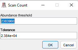
Figure 58: Threshold and tolerance dialog for the abundance distribution plot.
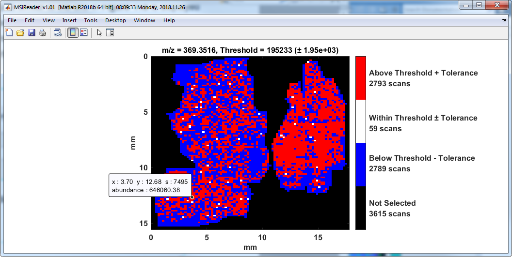
Figure 59: Abundance distribution relative to user defined threshold.
7.4.6 MSiSlicer
Selecting MSiSlicer in the pull-down menu, the current heatmap is loaded into a new GUI called MSiSlicer. The cursor immediately changes to a  , and the user can draw a segmented line ROI across the image. As shown in Figure 60, MSiSlicer then displays the ion abundance (bottom) along a segment line in the lower plot window. Black x’s mark the positions of the connecting points in the ROI. As the line is moved or the points edited the ion abundance plot is automatically updated. Three plot styles: line, stem and stairs, can be selected from a pull-down list. A checkbox locks the vertical axis of the plot and prevents the axis from automatically updating to accommodate the changing abundance range as the line is moved. The left panel of the GUI also contains information about the applied slice and tools to invert the heatmap colors, refresh the plots and redraw the ROI. The colormap can be edited by right-clicking on the colorbar to the right of the heatmap.
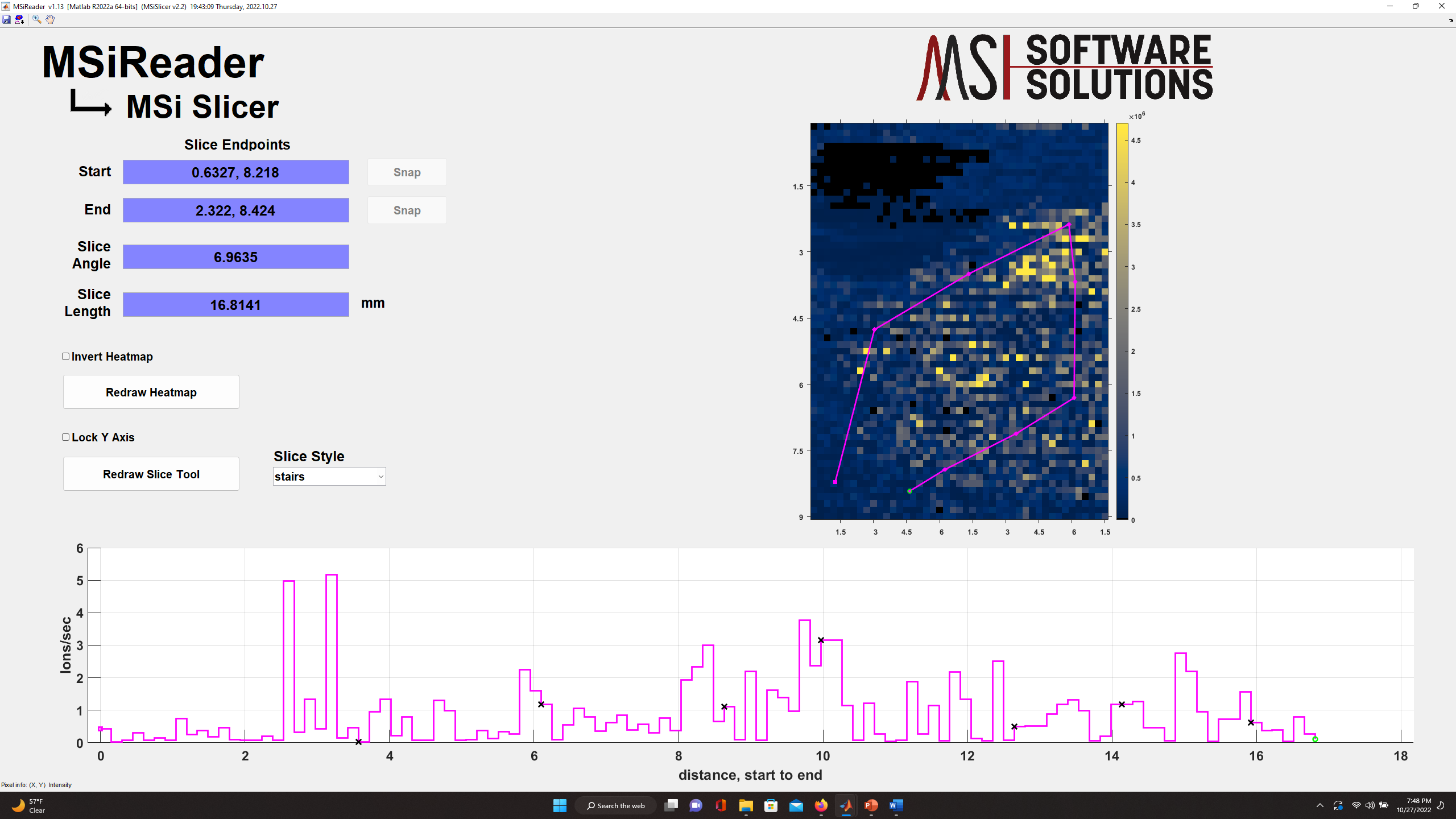
Figure 60: MSiSlicer GUI showing a “stairs plot” of the abundance of cholesterol across this tissue.
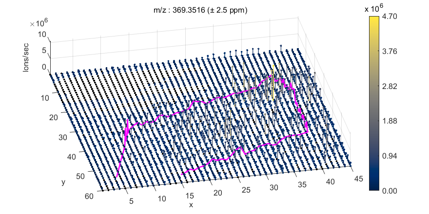
Figure 61: 3D Heatmap extracted from MSiSlicer.
By pressing the  icon in the MSiSlicer GUI, the heatmap will be extracted as a 3D figure where abundance is simultaneously represented as a heatmap and as an elevation on the z axis as shown in Figure 61. The plot shown is a 3D stem plot. Either stem3 or surface can be selected in the preferences INI file (§5). The view of the 3D heatmap can be rotated by clicking on the
  icon and then dragging the pointer over the figure. In addition to the 3D heatmap, the ion abundance plot is also extracted into a new window. Both figures can be saved to another format (e.g. .jpg, .png) from the File/Save as menu or saved as Matlab .fig files.
The data used to generate the 3D heatmap and the graph can also be extracted into an Excel workbook by clicking the  icon on MSiSlicer’s toolbar. In addition to information about the data set, the workbook will contain the raw heatmap ion abundance data as a matrix and the interpolated data used to generate the ion abundance plot (scan location and abundance vs distance along the segmented line) in separate worksheets. The exported heatmap data matrix can be read back into MSiReader as a custom abundance heatmap and used for normalization. Using this approach, you can normalize an image to a reference peak from another image, provided the images are the same size.
7.4.7 Image Overlay
The MSiImage tool can be used to combine another image with the heatmap, for example, an optical image of the same tissue. We recommend using third party tools to prepare your optical image prior to importing it into MSiReader; our tool works on editing images but it not overly sophisticated. The image can be in any graphics file format that Matlab can read (e.g., png, jpg, tiff) and any image can be used as the overlay including an exported heatmap plot for a different m/z value or even another tissue sample.
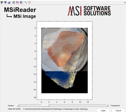
To use the tool, click on Image Overlay in the drop-down Visualization menu. This will open the MSiImage interface containing the current molecular image in the main MSiReader GUI as shown in Figure 62. After pressing the  icon, the user is asked to select an optical image file which will be resized to fit within the axes and displayed on top of the heatmap as shown in Figure 63.
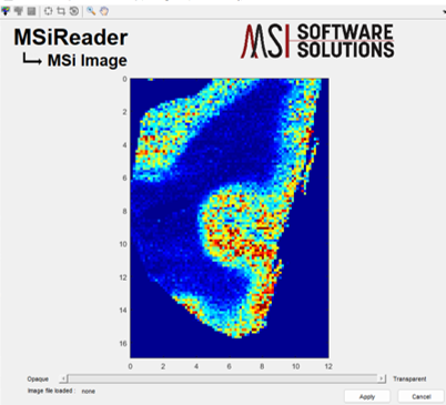
Figure 62: MSiImage loaded with current heatmap (m/z = 329.2475).
Figure 63: MSiImage after inserting an optical image (no alignment as been done at this stage). The toolbar contains icons to resize, crop and rotate the optical image overlay. Transparency of the optical image can be adjusted with the slider bar at the bottom.
The overlay image can be aligned with the underlying heatmap using the adjustment icons on the MSiImage toolbar. They are move/resize 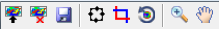 , crop and rotate . It is recommended to crop your image prior to loading or do that first using the tool in MSiReader. The image aspect ratio is 1:1 and locked by default but it can be unlocked by right-clicking on the heatmap after selecting the move/resize tool. The zoom and pan tools remain functional while adjusting the overlay. The rotate tool rotates the image about its center using mouse motion as input. A motion magnification factor, ImgRotateMag, can be set in the preferences INI file to speed up or slow down the rotation (§5).
Transparency of the optical image can be adjusted at any time using the slider bar at the bottom. After you are satisfied with the alignment and any resizing or cropping you have done the resulting image overlay can be saved for future use by clicking on the save icon  as a .png file. The .png file contains the image as seen in MSiImage. The image overlay can be removed by clicking the icon.
Upon clicking the Apply button, the MSiImage tool will close and the optical image combined with the MSI data will appear in MSiReader as shown in Figure 64. A transparency slider bar is added to the MSiReader main window under the m/z slider bar.
All MSiReader tools are fully functional with the overlaid optical image (browsing, data extraction, MSiPeakfinder, batch processing of images, etc.). Transparency of the optical image can be readjusted at any time using the bottom slider bar in the main MSiReader interface. Hint: You can make the optical image temporarily disappear by making it 100% transparent. Alternatively, the user can click on Remove overlay in the main MSiReader GUI on the bottom right-hand corner.
At any time, the user can press the MSiImage button again to realign the optical image, erase it, save it, or load a new one.
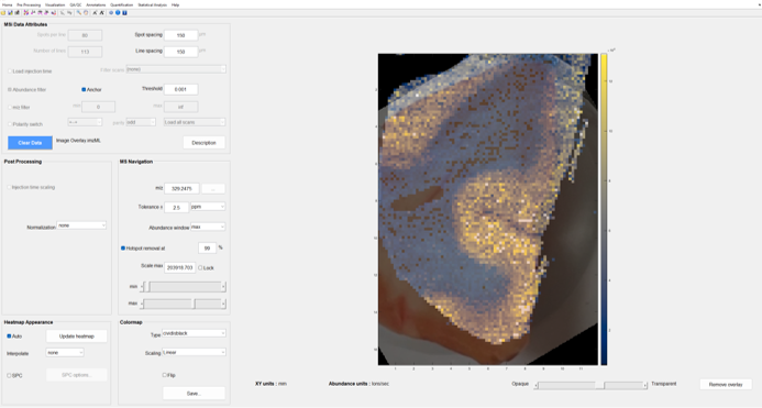
Figure 64: Overlaid optical picture and molecular ion map. The overlay transparency level is adjusted using the slider bar. To remove the image overlay, click on remove overlay on the bottom right-hand corner. This is NOT a toggle, once removed the user will have to go back into the image overlay tool to recover it. However, to temporarily hide the optical image, move the slider bar to 100% transparent.
7.4.8 8-Color Colocalization Plots
A video tutorial on generating colocalization color plots can be found HERE.
The user can overlap up to eight heatmaps using the color channels in MSiReader. Spatial overlap is often used to perform qualitative comparison of the distribution of specific molecules over the sample surface. To create a colocalization image, save figure (.fig) files for up to 8 individual heatmaps that you want to overlap. Any interpolation scheme, hotspot removal, tolerance, etc. can be used provided that these are the same for all the figures. When all the images are saved, select Colocalization Plot in the drop-down visualization menu to launch the colocalization interface. Using the interface, select a color to apply and browse to choose the corresponding figure file (See Figure 65); the red color channel is automatically selected and the remaining 7 channels can be enabled by checking the box next to them. If the user only selects the red, green and blue color, the default setting is to normalize channels separately and produce a blended plot of the channels that the user has chosen. However, the end-user can also change the normalization to max of all channels at which time a slider bar to change the gain for each of the three colors. Moreover, the plot mode can also be changed from blended to dominant mode; a dominant plot means that whatever m/z value is dominant in that pixel, that color will be displayed. If the end-user adds additional colors beyond red, green and blue, the plot is fixed and will produce a dominant plot of the color channels that are normalized separately.
Note 1: Separate .fig files are used as the input so users can integrate complex normalized heatmaps or custom heatmaps into colocalization plots.
Clicking the  icon will save the colocalization plot as a .fig file with relevant information in the title.
Another image can be overlaid on the colocalization heatmap using the toolbar icons for loading, deleting, moving, resizing, cropping and rotating. The slider bar at the bottom of the MSiColocalization GUI can be used to adjust the opacity of the overlay once an image is loaded. See §7.4.7 for details on using the image overlay tools. The slider bar is only displayed if an image file is loaded to map to the mass spectrometry imaging data.
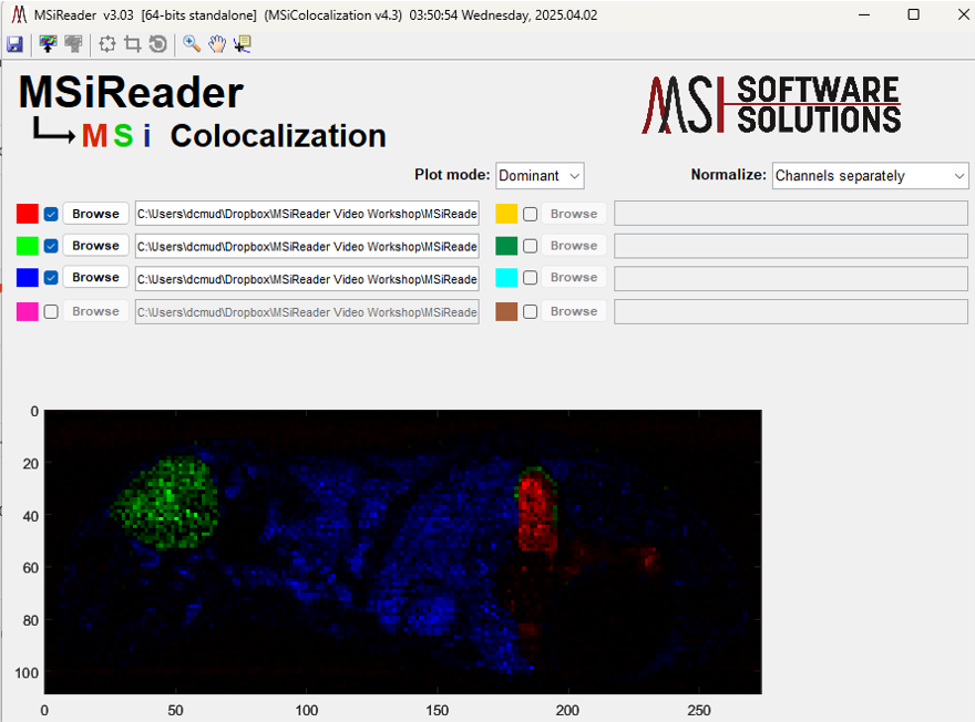
Figure 65: MSiColocalization interface showing three m/z values on a whole mouse tissue imaging dataset (red channel is m/z = 303.2531, green channel is m/z = 367.3301 and the blue channel is m/z = 617.1808. The default is to normalize each channel separately in blended mode and this is what is shown.
The data for each color channel is divided by a normalization scaling factor and multiplied by a gain. The gains are initially set to one and the slider bars for relative color intensity range logarithmically from 0.00001 to 100000. The channel normalization factors can be selected with the right-click context menu in the Gain panel in MSiColocalization as shown in Figure 66 (right-click on the word Gain to access this menu). None means that the data is not normalized (i.e., the scaling factor is unity). The other two choices normalize each channel to its maximum abundance value or globally to the maximum abundance in any of the data sets. When the normalization method is changed the colocalization plot is immediately updated. The default method can be set in the preference INI file with the ColocalNormOption value (§5).
Note 2: The figure files do not have to be the same size. The smaller figures will be resized to match the largest one. The maximum allowed size difference in either the column or row dimension is 80%. This value can be changed in the preference INI file (§5).
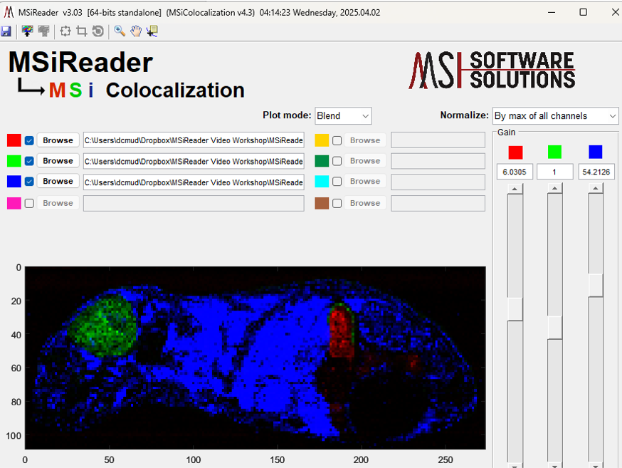
Figure 66: Color channel normalization menu. Click on “Normalize” and choose from None, Channels Separately, or Max Abundance in all channels.
Note 3: DO NOT use .fig files that contain drawn ROIs or image overlays. The user can add image overlays after the co-localization plot is made using the icons in the toolbar in the co-localization GUI.
7.4.9 3D Plotting
For a video tutorial on how to generate 3D Heatmaps, click HERE.
Three 3D plots are available by selecting 3D Plotting from the drop-down menu. The choices are mass spectra plot, an image stack and a 3D colocalization plot. The spectral plot is either a waterfall line plot or stem plot for a selection of previously exported centroid or average spectra. The image stack plot is either a stack of spatial heatmaps, one each for a list of m/z values or a stack of spatial heatmaps, one each for the files in an image mosaic. 3D colocalization plots are a stack of image layers, one each for a set of previously saved .fig files created by the MSiColocalization tool.
7.5.1 Mass Measurement Accuracy
A video tutorial on the use of the MMA QA/QC tool can be found HERE.
MSiReader provides tools for the calculation and plotting of mass measurement accuracy (MMA) for any m/z in an ROI or for the entire image. Access this tool by selecting Mass Measurement Accuracy under the QA/QC menu. For a given m/z and tolerance, MSiReader finds the most abundance peak, max_peakk, in each scan that is within the tolerance window. It then calculates the MMA for each scan as,

After the MMA value is calculated for all scans in the ROI (or image), several types of plots can be produced or the MMA data can be saved into an Excel or text file. The submenus for the MSiReader heatmap axes have seven items for selecting these MMA functions as shown in Figure 67. Each is described below. Note that if an ROI is active when an MMA function is invoked the user is prompted to select either all the scans or only the ROI scans for processing.
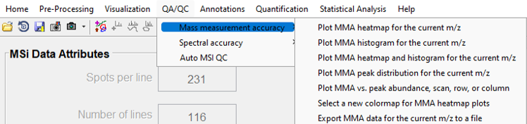
Figure 67: Mass measurement accuracy drop down-menu choices (described below).
7.5.1.1 Plot MMA heatmap for the current m/z
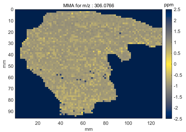
Figure 68: MMA heatmap for m/z = 306.0766
A mass measurement accuracy heatmap for the current m/z center value and tolerance is displayed in a new figure. The color of each pixel in the exported heatmap is proportional to the MMA value of the most abundance peak in the m/z window. The default colormap used for the plot is a balanced colormap with the most intense color in the center where the MMA equals zero and the least intense color at the plus and minus limits of the m/z tolerance (set these in the main GUI for MSiReader). The colormap used for the MMA heatmap is specified by a preferences INI file variable MMAColorMap (§5). The default colormap is parulahi.mat. An example of this plot is shown in Figure 68.
The MSiReader installation folder includes the default colormap as well as a parula based colormap with the highest intensity at the m/z tolerance limits and the lowest intensity at the center value. It is named parulalo.mat. Balanced versions of six other colormaps are also in the colormap folder, \msicolormaps.
The data tips tool (“transparent menu” above the heatmap, second from the left) can be used to query the spatial coordinates (X, Y, and scan number), the MMA value and the most abundant peak (m/z and abundance) that was used to calculate MMA for that scan.
7.5.1.2 Plot MMA histogram for the current m/z
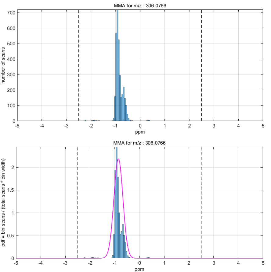
Figure 69: Mass measurement accuracy histogram and probability density function.
Two histogram plots are produced. One shows the number of scans in each ppm bin and the other normalizes the bins counts such that the height of each bar is proportional to the number of scans in each bin divided by the product of the total number of scans and the bin width (i.e., the probability density function or PDF). The area of each bar is the relative number of observations. A Gaussian normal curve with the mean and standard deviation of the binned data is also plotted on the probability density histogram. An example of these two plots in Figure 69 shows a systematic mass shift of -0.9 ppm.
Two preferences INI variables (§5) control the histogram bar direction, MMAHistogramDirection, and the bin selection method, MMAHistogramBinMethod. The default values are vertical and auto. The bar direction can also be horizontal as shown in Figure 70.
By default, the histogram has the same m/z window size as the heatmap. However, the m/z window for the histogram can be extended (by a multiplicative factor) to reveal any significant values outside of the tolerance window. This is done by setting the MMAHistogramMargin variable in the INI preferences (§5) file to rescale the m/z window for the histogram calculation. The default value is 1 ppm.
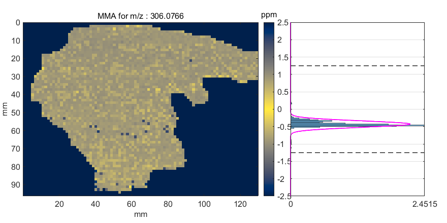
Figure 70: Mass measurement accuracy heatmap and histogram. Please note that the heatmap uses the scale from 2.5 ppm to -2.5 ppm while the histogram goes from 5 ppm to -5 ppm (the dashed lines are the ± 2.5 ppm limits) but the values are not listed on the dual plot as it becomes too crowded.
7.5.1.3 Plot MMA heatmap and histogram for the current m/z
This plot is a combination of the first two plots; a mass measurement accuracy heatmap and a PDF histogram. The histogram is oriented in the horizontal direction. Elements of this figure can be moved, resized or deleted using the figure toolbar edit tool (left leaning arrow). If the MMAHistogramMargin Preferences INI (§5) value is larger than one, the histogram window is extended as described above. The dotted lines in the figure delimit the m/z window used to calculate the MMA and the limits of the plot show the additional margin value described above.
7.5.1.4 Plot MMA peak distribution for the current m/z
An animated scatter plot is drawn showing the distribution of MMA vs ion abundance for all peaks in the m/z window. The animation is by scan number and the pixels for each scan have the same color. The data tips tool (“transparent menu” above the heatmap, second from the left) can be used to query the spatial coordinates scan number, MMA and abundance.
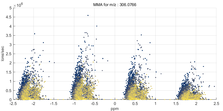
Figure 71: Mass measurement accuracy peak distribution.
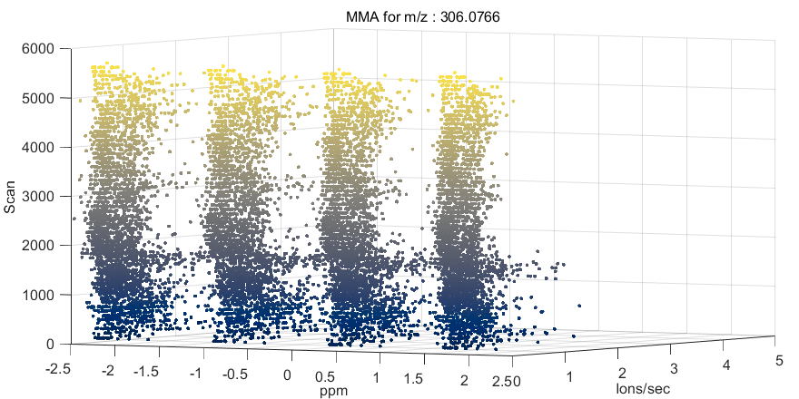
Figure 72: Mass measurement accuracy peak distribution by scan.
Note 2: The mmaabundance and mmadistribution plots are 3D plots viewed from above the XY plane. The Z direction is the scan number. This can be seen by using the figure toolbar rotate icon to change the viewing angle. After enabling this tool, the right-click context menu can be used to quickly view the data relative to the XY, XZ or YZ planes. For example, when Figure 71 is rotated as shown in Figure 72, not only is the MMA clustering visible, but it can be seen that the MMA shifted (-) and then (+) slightly as the sample was scanned.
7.5.1.5 Plot MMA vs. peak abundance, scan, row, or column
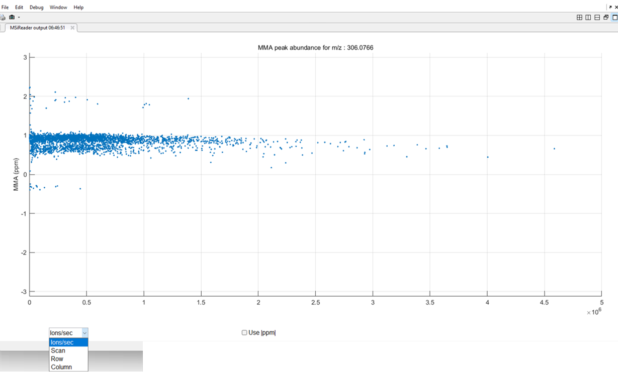
Figure 73: Mass measurement accuracy as a function of the ion abundance of a specific m/z value.
A scatter plot is produced with a point for each scan showing the abundance vs MMA values used to produce the MMA histogram. This is the raw data that is used to make the histogram plots. The data cursor tool can be used to reveal the scan number, MMA value and abundance for any point. There is a drop-down menu on the bottom left of Figure 73 for which the end-user can select ions/sec (abundance), scan number (time), row or column. This sets the x-axis accordingly. Moreover, if the user wishes to make a plot where the y-axis is absolute MMA (the direction of the MMA does not matter), click the “Use ppm” checkbox in Figure 73.
7.5.1.6 Select a new colormap for MMA heatmap plots
Allows the user to select a MMA heatmap colormap of their choice. Most of these will not be bi-directional. In other words, going to + MMA values will be a different color than going to – MMA values.
7.5.1.7 Export MMA data for the current m/z to a file
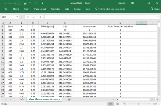
Figure 74: Mass measurement accuracy data exported to an Excel file.
The MMA heatmap data is calculated and exported to an Excel workbook or a text file if Excel is not available. Included for each scan are its X and Y location, the MMA value in ppm, the m/z and abundance of the maximum peak in the m/z window and the number of data points in the window. An example of exported MMA data is shown in Figure 74.
7.5.2 Spectral Accuracy
A video tutorial on how to use the spectral accuracy QA/QC tool can be found HERE.
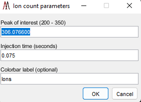
Figure 75: Isotope ratio parameters dialog.
Access the spectral accuracy (atom counting tool) by selecting Spectral Accuracy in the drop-down menu under QA/QC. This will give the user two different pieces of data. The first, Plot ion count heatmap, produces an ion count plot for an m/z, which is the heatmap data scaled by injection time. Access this function by selecting “Spectral Accuracy” in the pull-down menu and then “Plot ion count heatmap”. If ROIs are active, the user is prompted to select either ROI scans or ALL Scans. The user is then prompted to enter an m/z value (peak of interest), the injection time, and a colorbar label (Figure 75). The plot is the same if a user exported a heatmap in the main MSiReader GUI if injection time was loaded along with the data set. An example is shown in Figure 76. This output shows absolute number of ions in a heatmap as it has been shown that spectral accuracy is related to the abundance16. This can be used in conjunction with the plot isotope count heatmap (see below).
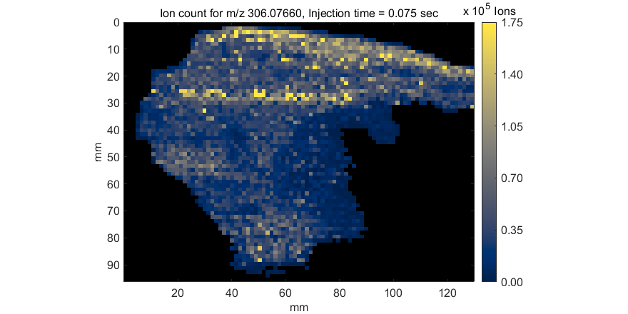
Figure 76: Exported ion count heatmap.
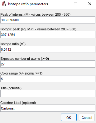
Figure 77: Dialog box for determining the accuracy of counting atoms.
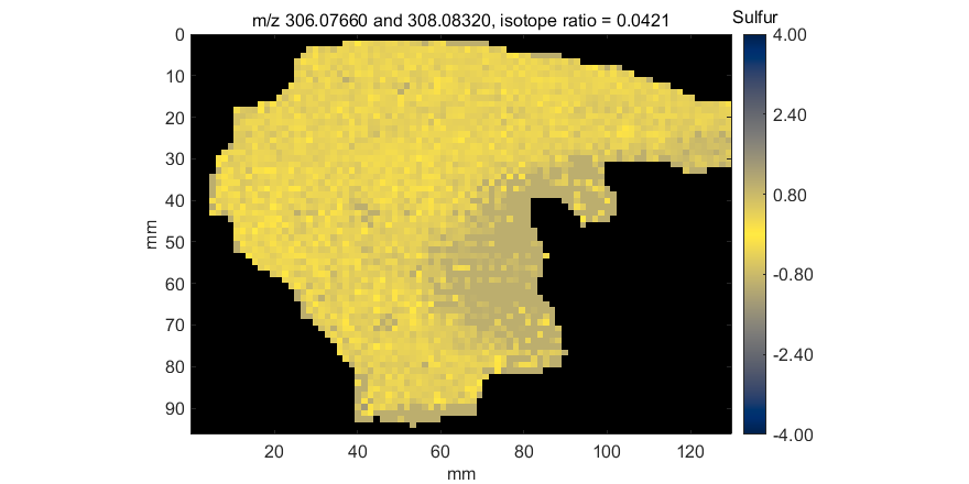
Figure 78: Heatmap showing the deviation from the expected number of sulfur atoms and that supported by the data. In this example, the expected number of sulfur atoms is 1.
The second option in the pull-down menu is Plot isotope count heatmap, which compares the ratio of abundance for two m/z values (e.g., the monoisotopic m/z (M) and the M+1 peaks of an atom) against the known ratio of those two isotopes. The dialog shown in Figure 77 is launched for the user to enter two isotopes, the abundance of the heavier isotope, the expected atom count, a tolerance range and optional labels. Once all user input is entered, select OK and then a heatmap will be displayed (which can be saved) and the user will be prompted to enter a filename (abcd.xlsx) to save the metadata as well as the spectral accuracy data in Excel format in two different worksheets.
A heatmap plot showing the deviation from the expected number of atoms at each scan is displayed (Figure 78). Note that the spectral accuracy is, in general, very good (yellow means that the deviation from the expected number of atoms is zero); however, the region on the right center of this tissue does not do as well as the rest of the ROI – this is attributed to higher ion abundance of this molecule on the left-hand side of this tissue than on the right (see Figure 76).
7.5.3 AutoQC MSI
Summary statistics for all tiles in a multifile image mosaic for each m/z value in a list. The results are saved into an Excel workbook with the following 16 worksheets.
Info Folder, date, version, settings, and options
File File names in the selected folder
Tile Sum Abundance sum
Tile Max Maximum abundance
Tile Mean Mean abundance of scans above threshold
Tile Std Dev Standard deviation of scans above threshold
Tile RSD RSD of scans above threshold
Tile Mean Zero Mean including low abundance scans
Tile Std Dev Zero Standard deviation including low abundance scans
Tile RSD Zero RSD including low abundance scans
Tile MMA Mass measurement accuracy
Tile Isotope Count Spectral accuracy for the isotope peaks
Tile Detection Frequency Ratio of scans above threshold to total number of scans
Tile Iso Detection Frequency Detection frequency for the isotope peaks
Tile Num Scans Number of scans above threshold
Tile Iso Num Scans Number of scans above threshold for isotope peaks
The current MSiReader Navigation panel values are used to generate abundance matrices for each m/z and isotope peak. The Info worksheet contains the current options, m/z values, isotope data and thresholds used to create the results. Each peak of interest and each isotope can have a different abundance threshold. The results worksheets contain a value for each m/z and each file. They can be arranged with file data down the columns or across the rows.
AutoQC MSI is an algorithm to compile a significant number of statistics on a folder of data for which the expected answer is known. This is evolving into a system suitability testing approach and will be in a future release. First, this function only works for a folder of files so the first step is for the user to load 2 or more files in MSiReader. Next, from the pull-down menu, select AutoQC MSI. The dialog box shown in Figure 79 will pop-up. In this example, the molecular formula of the molecule is C13H12F2N6O.
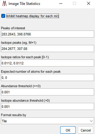
Figure 79: AutoQC MSI dialog box.
Here the user will enter in the peak(s) of interest, isotope abundance of the heavier isotope (13C = 0.0112), isotope ratio that is expected, number of atoms for each peak, abundance threshold, isotope abundance threshold and how the results should be output (tile or m/z). The user will then be prompted to enter a filename for the result will be in Excel format. The output gives a lot of basic statistics for each file that was loaded (for each peak of interest and its isotope) including the mean, RSD, isotope count, detection frequency, and number of scans the peak was found in (must be above the user set abundance threshold for both the peak of interest and its isotope threshold abundance (e.g., 13C). These can be useful QC statistics (even in raw format) to make sure that your MSI platform is operating properly.
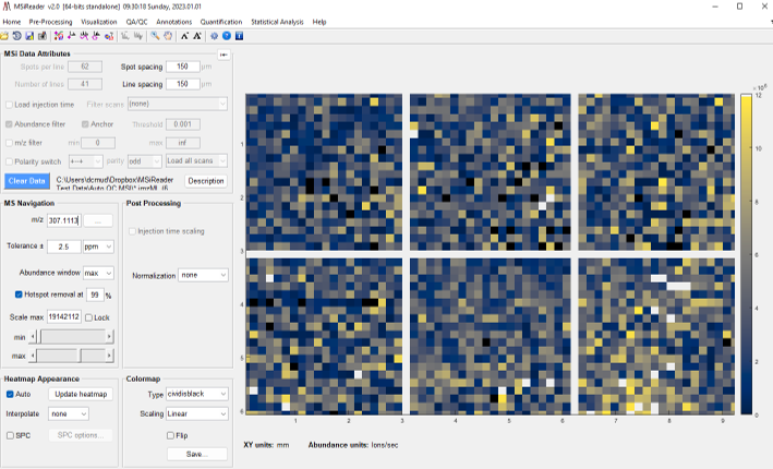
Figure 80: Loading of 6 QC ROI’s into MSiReader. The peak of interest is m/z = 307.1113 with a M+1 peak (m/z = 308.1147).
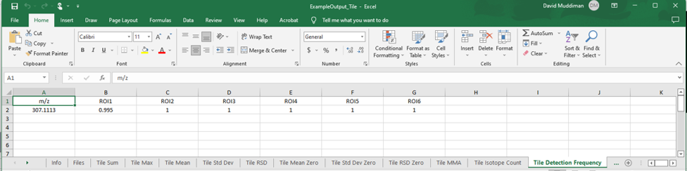
Figure 81: Example of data (summary statistics) generated from the Auto QC MSI tool. This is an example spreadsheet that shows the data for detection frequency for each ROI, each containing 400 voxels, that were measured. In this case, 5 out of the 6 ROI’s detected the compound in every single voxel while in ROI1, the data indicate it was detected in 398 out of 400 voxels which equates to a detection frequency of 0.995.
For example, six ROI’s were collected where each image was 20 × 20 pixels (voxels) with a QC standard homogenously sprayed on a glass slide (data shown in Figure 80). These were loaded into MSiReader and processed as outlined above using tile as the output setting (enter “1” in the dialog box shown in Figure 79). Figure 81 shows an example of the data output to an Excel spreadsheet when using this tool.
7.6 The Annotations Menu
There are several ways to annotate data in MSiReader which include the MSiSpectrum tool, the MSiPeakfinder tool, and the Search Custom DB tool. The first two use the current dataset loaded into MSiReader to search while the Custom DB tool can annotate a file from any source provided it is in the correct format. It is important to note that the default databases (MSiReaderPositiveIons and MSiReaderNegativeIons) are NOT loaded when MSI Reader starts. The user can change the default settings in the preferences .INI file (§5) to load them when MSiReader is started. Alternatively, the user can right click on the MSiReaderPositiveIons or MSiReaderNegativeIons and click on Reload. This is true for all three ways to annotate a dataset. For MSiSpectrum and MSiPeakfinder, the user has to select a ROI (two for MSiPeakfinder) to generate the .xlsx file while the search Custom DB tool does not require data to be loaded as this is annotating a file that was previously exported.
7.6.1 Database Searching
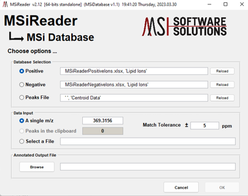
Figure 82: MSiDatabase GUI. Selection is for a file that was generated in this example using MSiSpectrum – in this example the filename is Mouse ROI.xlsx.
A tool for searching a results file in Excel format to find matches for a list of putative m/z can be selected by choosing Database under the Annotations menu and then Search custom database in the sub-menu. This will launch the MSiDatabase tool shown in Figure 82. Note that you must first use MSiExport, MSiSpectrum or MSiPeakfinder to generate the results file from your imzML file. It allows the user to annotate a single peak (the default for this field is the current m/z value in the main MSiReader GUI but it can be edited), the peaks in the clipboard, or the user can select a file. The file could be a previously exported results file from a peak picking session or any Excel worksheet containing a list of m/z values in the first column.
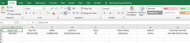
Figure 83: Output using the Custom DB annotation tool with a query for a single m/z value. Note that the only the information about the single m/z is included in the output.
To annotate a single m/z value that maybe present in your data, enter the m/z value in the Mass Selection pane as shown in Figure 73 along with a Match Tolerance in ppm. In this way, the dataset that you have exported into an Excel spreadsheet will be annotated. For the mouse dataset, enter 768.5514 and load the File to Annotate (Mouse ROI.xlsx). The output from the single m/z query is shown in Figure 83.
The user can select the Select a File radio button (Figure 82) and then a dialog is launched for the user to choose an Excel file. If the selected file contains multiple worksheets, a prompt is issued to pick the correct one. In each scenario, the user can also choose a m/z match tolerance and a database that is for either positive or negative ionization mode.
Importantly, an alternate database file can be loaded at any time by right-clicking on the positive or negative mode file name and a dialog will be launched that says “reload positive ion database” or “reload negative ion database”. This can be custom made by the end-user specific to their project. The default databases can be set in the Preferences .INI File (§5). Or simply click “Reload” next to the relevant database.
For the example shown, a positive-ion mode data file has been selected as the m/z source which contains a large number of m/z values. In this case, the output location and filename has defaulted to be the same filename. The user can click the Browse button to select some other output file (including a new empty file). In either case, information from the database is always added to output file in columns to the right of any existing columns. This allows the user to annotate a previously annotated file without overwriting information. For example, after a database has been updated, an old file could be processed by MSiDatabase again to search for new matches.
Figure 84 shows an annotation of the Centroid Data worksheet from a previous export of the MSiSpectrum tool. The first two columns are the original output results. The next two columns with light blue background contain the m/z keys from a positive ionization database that match within 5 ppm and the MMA calculation for each match. The five columns with light tan background were copied from the database file for the matching keys.
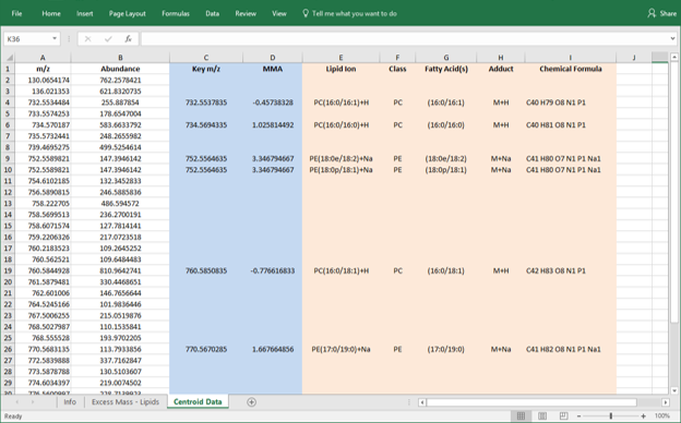
Figure 84: An example of the annotated file using a data export from MSiSpectrum.
If the mass source was a single m/z or a list of peaks in the clipboard, then the output file will contain the query m/z values in the first column. Any matching database keys, MMA and annotation information would follow in columns two through eight.
The MSiSpectrum and MSiPeakfinder tools have checkboxes in the Peak Export (centroided data) panel that enable the database annotation and tolerance selection in addition to the other options for exporting results. In this case, the Centroid Data worksheet is annotated as soon as it is created without the need to run the MSiDatabase tool separately. Figure 85 shows the annotation functionality in the MSiSpectrum tool. The user should check Use Database to Annotate Peaks to annotate the data during the export.
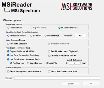
Figure 85: The annotation tool as deployed in the MSiSpectrum tool.
The preferences INI file (§5) has variables for the name and format of each database Excel file. The format of each is specified with six values: a worksheet name, the column containing m/z key values, a list of the information column numbers to be added to an annotated worksheet, the row number containing labels for the information columns, and the first row that contains data.
Example databases are provided with the MSiReader distribution. There are files for positive and negative mode ionization from a shotgun lipidomics study which can be used as an example of how a user might build their own database with ions of interest; one for positive ion mode and one for negative ion mode.
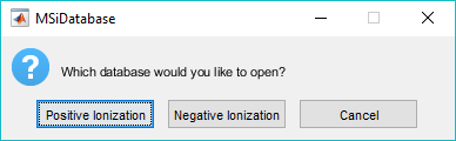
Figure 86: Ionization database selection dialog to open an existing database and make additions to it.
One can make additions to an existing file simply by clicking Database in the pull-down menu and then selecting “add record to database” from the Annotations menu. Upon doing so, an ionization selection dialog box shown in Figure 86 and then opens the current database file for the selected mode in Excel. A user can make edits / additions and then have an option to save or not save those changes.
7.6.2 Molecular formula adduct search
A video tutorial on using the molecular formula tool can be found HERE.
An isotopic distribution and adduct calculator, MSiFormula, can be launched from the drop-down menu by selecting molecular formula adduct search. The MSiFormula GUI is shown in Figure 87. A formula can be entered using the standard names of the first 92 elements of the periodic table and the theoretical monoisotopic mass and isotopic distribution will be automatically calculated using the NIST standard table of stable isotopes. Inclusion of heavy isotopes can be entered explicitly (for example, 13C2 or 15N4) and the exact mass those isotopes will be used when calculating the isotopic distribution. The mass of any occurrence of an element not preceded by an isotope number will be found using the stable isotope distribution table. A context menu on the molecular formula entry box allows an immediate change of the 13C or 15N ratio for this session of MSiFormula. The ratios of 12C and 14N are automatically adjusted so the ratios sum to one for each element.
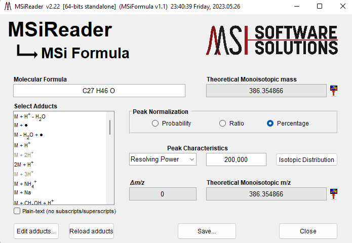
Figure 87: MSiFormula GUI for finding adducts of a given neutral molecular formula in a loaded dataset.
Elements may be entered in any order and may occur multiple times. An element name not followed by a numeral is assumed to occur once. The elemental parts of a formula must be separated with whitespace when an isotope is used. For example, the formula “13C15N18O” without whitespace could be interpreted as “13C15 N18 O”, “13C15 N 18O”, “13C 15N18 O”, or “13C 15N18 O”.
The peaks of the isotopic distribution can be normalized so their heights sum to one (probability), so the most abundant peak is one (ratio), or so the most abundant peak is 100 (percentage); the default is percentage. The theoretical isotopic distribution can be plotted with the peak shape specified by a single numeric value, either full width half max (FWHM) or mass resolving power – simply click the isotopic distribution button. The isotopic distribution is carried out using the Fourier transform methodology17. Either a line or stem plot can be drawn, with or without peak markers and a legend with menu options on the plot button. The theoretical monoisotopic mass can be sent to the MSiReader navigation panel and the heatmap will automatically be updated.
A pull-down list of common adducts is available to modify the isotopic mass of the formula. If multiple adducts are selected, multiple results will be displayed as expected monoisotopic masses. Any of these results can be sent to the MSiReader navigation panel to immediately update the heatmap.
The adducts are stored in an Excel workbook named, MSiAdducts.xlsx, in the MSiReader installation folder. It contains 35 positive mode adducts and 15 negative mode adducts. The file can be edited to add, remove, or change the order of the adducts. The names of the adducts are arbitrary and will appear in a list selection in MSiFormula. The columns of the Common Adducts worksheet needed by MSiFormula are described by a set of preferences INI file variables (§5). Other columns in the worksheet are ignored.
Variable Value
AdductCalculatorFile MSiAdducts.xlsx
AdductCalculatorWorksheet Common Adducts
AdductCalculatorLegend Legend
AdductCalculatorHeaderRow 1
AdductCalculatorFirstRow 2
AdductNameColumn 1
AdductModeColumn 2
AdductFormulaColumn 3
AdductChargeColumn 4
AdductMultiplierColumn 5
AdductDeltaMassColumn 6
AdductDefaultSelection 0
The results for a molecular formula (masses, ratios, and isotopic distribution) and all selected adducts can be saved into an Excel workbook. Multiple instances of MSiFormula can be run simultaneously and data does not have to be loaded into MSiReader prior to launching the tool. Multiple default adducts can be specified with a vector of row numbers in the Common Adducts worksheet for the value of AdductDefaultSelection. Zero means that no adducts are initially selected.
If you want to add to the adducts, click Edit Adducts and the Excel spreadsheet will open. Make edits and save the spreadsheet using the same file name. Then click Reload Adducts so it re-reads the file. Those options will now appear in the window.
To determine how a molecule ionizes (e.g., M+H+ or M+Na+), enter in the molecular formula and select the adducts you want to be considered. This will automatically populate the fields Dm/z and Theoretical Monoisotopic m/z. Next, click the ICON to the right of Theoretical Monoisotopic m/z – this will pop up a window with the m/z values of the different adducts under consideration. If you only selected one adduct, it will automatically update heatmap with that single m/z value. Repeat this process for each m/z (adduct) being considered and make note of the abundance of each type of adduct. This tool can be very effective at determining how a molecule ionizes.
7.6.3 SSIM Colocalization Tool and Batch Processing
7.6.3.1 Background Information
Navigating large data sets and generating heatmaps for more than a few m/z values can be tedious. MSiReader has implemented a batch processing feature to automatically generate and save a heatmap plot for all of the m/z values in a list. After selecting a source of peaks and a destination folder, images are generated (default is a .png file) and saved for each peak. Thousands of image files can be created in less than an hour and rapidly sorted by the user later using any graphical image viewer software. This is particularly useful to visualize the output from the automatic peak picking function. It is also very handy for users who want to quickly extract images for a list of target m/z values and for peaks that are found and saved while navigating the data set. The source of the m/z values can be the contents of the clipboard, an Excel worksheet, a text file, or a sequence of values uniformly spaced over an m/z range. If an Excel workbook is selected that has more than one worksheet, the user is prompted to select the correct one. The m/z values in the first column of the selected worksheet will be used as the peak list.
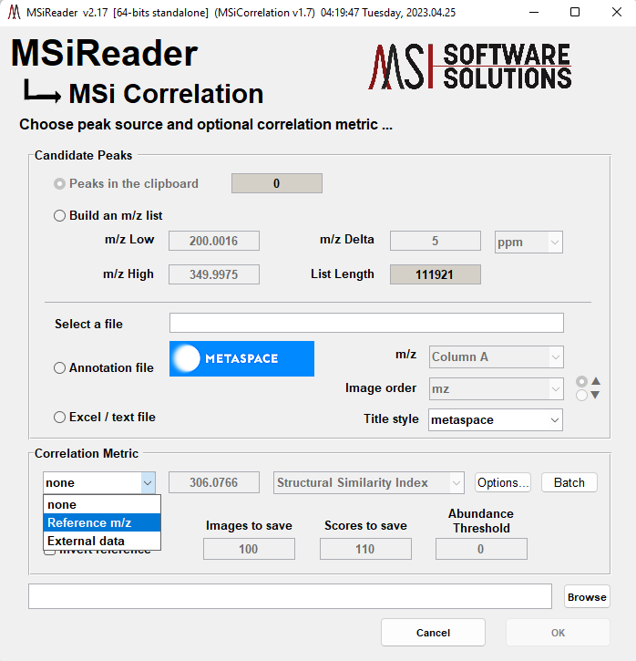
Figure 88: The correlation and batch processing user interface in MSiReader.
Batch image processing has been incorporated into the image correlation tool which is launched by selecting SSIM co-localization tool under the Annotation menu. The MSiCorrelation GUI is shown in Figure 88.
MSiCorrelation generates a folder of images in exactly the same way as the batch processing tool if the Correlation Metric pane pull-down selection is none. Images in the format described below in §7.6.5 will be saved in a folder selected by the user. The files will be named after the m/z value of the image (e.g., the image for m/z 369.3516 will be saved as 369_3516.png) for easy sorting. The title information, figure size and colorbar characteristics can be customized with the preferences .INI variables (§5) shown in Table 4. Their meaning is identical to that described above for exported figures. However, note that default values are different for batch and figure export.
Table 4. Batch figure formatting options.
BatchFileType | png |
BatchFigureSize | system dependent |
BatchFigTitleStyle | batch |
BatchFigAxes | true |
BatchFigAxesLabels | true |
BatchFigColorbarStyle | compact |
BatchFigColorbarLabels | 6 |
BatchFigColorbarPrecision | 2 |
BatchFigFontName | Arial |
BatchFigFontSize | 12 |
ExportToMATBatch | false |
ExportToFIGBatch | false |
The additional settings for batch processing are set with preferences file INI variables (§5). They are: ExportDuplicateMZBatch, BatchPeakHeatmapUpdate, and BatchHeatmapVisible. The default value for all three is false. Setting them to true will cause duplicate m/z values to generate separate images, update the MSiReader heatmap as each value is processed, and make the separate figure window for each image visible as it is created. Enabling either of these last two settings will significantly slow down batch processing.
There is the option to generate a uniformly spaced list of values over any m/z range for batch processing and image correlation. Element spacing can be in absolute or ppm units. Current normalization and windowing selections from MSiReader are used when the images are generated. The m/z Delta value defaults to the current MSiReader window width. Increasing it will leave gaps between the windows and decreasing it will result in overlapping windows.
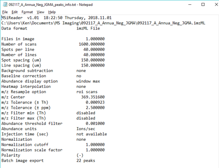
Figure 89: Example of the information saved as a text (.txt) file with a batch of images.
Other information relevant to the data set and options that were selected are saved into a short text file in the same folder as the images. An example is shown in Figure 89. A second text file is written into this folder containing the m/z peaks list. This later file can then be used as a peaks list for analyzing another data set. If the loaded data set was a folder of imzML or mzXML files a third file is saved containing the tiling pattern and a list of the file names. The default number of decimal places for the m/z value and the m/z window is 5 but can be modified in the INI file (§5) by changing the mzExportPrecision variable. If a photographic image overlay has been loaded, the overlay is included in each of the batch processing output files. The transparency slider can be used to temporarily hide this photo overlay without deleting it before launching MSiCorrelation. Recall that the color scale can be locked during batch processing so that the images all have the same abundance to color mapping. If the color scale is locked and a file containing an m/z peaks lists was selected that had a second column of values, then the user is given the option to use those values for the abundance to color mapping for each m/z. This is useful for generating images for an m/z target list that are visually comparable across multiple data sets with the same abundance range for all the images.
7.6.3.2 Image Correlation Algorithms
As shown in Figure 88 there are two other choices for the Correlation Metric pane pull-down selection, Reference m/z and External data. Either of these will result in the list of candidate m/z values being compared and ranked by their similarity to a reference image. If Reference m/z is chosen, the image data for the value in the data entry box is used as the reference. If External data is chosen, the user will be asked to select a .mat file containing one or two matrices with the same dimensions as the loaded set. The first matrix becomes the reference data, the second optional matrix is a binary mask that can be used to exclude a portion of the reference matrix from consideration. For example, scans outside of a tissue ROI. A special case of an external reference is the down sampled version of an optical overlay imaged saved with the MSiImage tool as described in Section 7.3.2. In this case MSiCorrelation automatically chooses the correct matrices in the .mat file.
The current MSiReader normalization and window settings are used when generating candidate images for correlation with the reference. The value in the Abundance Threshold data entry box can be used to exclude very low abundance images. This can be particularly useful when using a very large list of m/z candidates. If all of the scans for an m/z have ion abundances below the threshold, that image is considered empty and excluded. Note that this evaluation is done after applying normalization, thus it may be difficult to select an appropriate threshold value. It may be helpful to normalize to the maximum abundance so that all of generated images and the reference have an abundance range between zero and Normscale (§5).
An external data set that is used as the reference image may have already been normalized. In this case, uncheck the Normalize Data in the Correlation Metric pane to disable normalization of the reference image so that it is not normalized twice.
Three algorithms are implemented for scoring candidate images with respect to the reference. In Figure 90 the Structural Similarity Index has been selected from the pull-down list. The other three algorithms are Absolute Difference, Mean Squared Error and 2D.
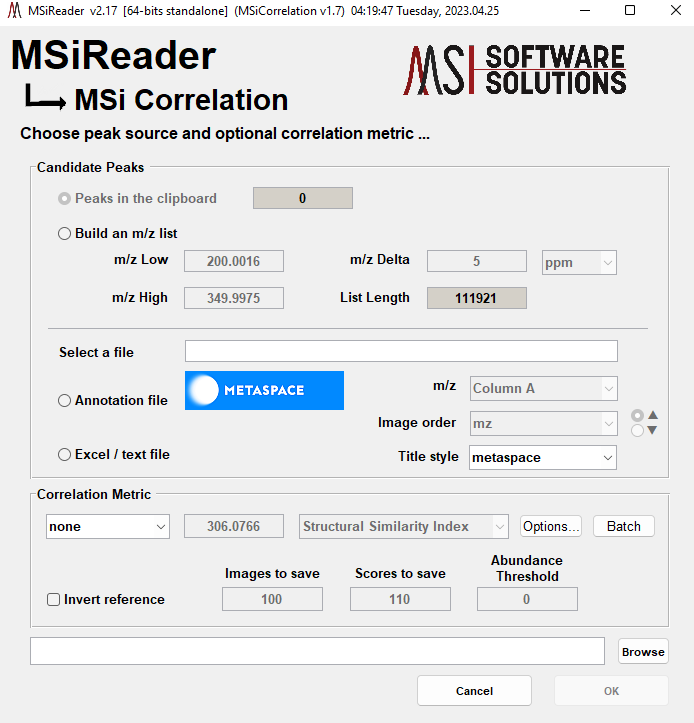
Figure 90: MSiCorrelation GUI showing selection of SSIM as the algorithm for image correlation.
The scoring algorithms for image correlation are:
Absolute Difference Subtract the reference image matrix from each candidate element-by-element and sum the absolute value of those differences. A score of zero means the images are identical.
Mean Squared Error The square root of the sum of the squared differences is divided by the number of elements. This is equivalent to the Euclidean 2-norm (i.e., the vector length) divided by the number of elements. A score of zero means the images are identical.
2D This was added to the MSiCorrelation tool as an optional scoring algorithm selection.
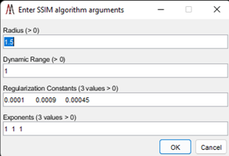
Figure 91: Parameters selection dialog for the SSIM algorithm.
Structural Similarity Index An index based on human perception of quality or image “likeness”. The SSIM algorithm18 was developed for digital image processing as a measure of the quality of images after compression, filtering, transmission and reproduction. The similarity measure of a reference standard against candidate images is the weighted product of the luminance, contrast and structural components of the image. The SSIM default parameters can be accessed in MSiReader by clicking Options to the right of SSIM in the correlation metric pane; the input values are shown in Figure 91; these were determined in a previous study to be optimal for MSI19.
The Radius parameter specifies the standard deviation of an isotropic Gaussian function used for weighting a window of pixels surrounding each pixel. The Dynamic Range parameter is the absolute range of values in the input images. The regularization constants are used to stabilize the luminance, contrast and structural components when the local mean or standard deviation in a small region tends toward zero. Lastly, three Exponents are used to adjust the relative importance of the luminance, contrast and structural components before combining them into a single score. While the default values work well, the user should refer to these references18,19 for more details. SSIM scores range between -1 and +1, with one indicating a perfect match.
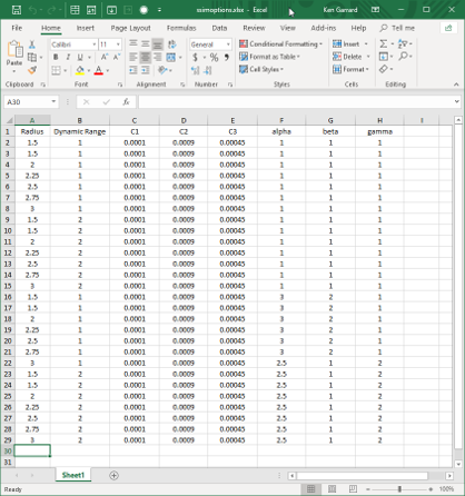
Figure 92: A file of parameters for SSIM image correlation. Each candidate image is evaluated with each set of parameters.
Choosing Batch to the right of SSIM in the Correlation matrix pane in Figure 90 launches a dialog for the user to choose a file of SSIM parameters. The file can be Excel or text format with each row or line containing the eight parameter values. An example is shown in Figure 92 with 28 sets of parameters varying the radius, dynamic range, and weighting exponents. MSiCorrelation will execute the SSIM algorithm using all combinations of parameter sets and candidate m/z values and rank them by their similarity score. Using this option allows for great flexibility in testing a large number of parameters for your specific dataset.
If ROIs are present in MSiReader when using MSiCorrelation, the user is prompted to select the scans of interest using one of the dialogs shown in Figure 93.
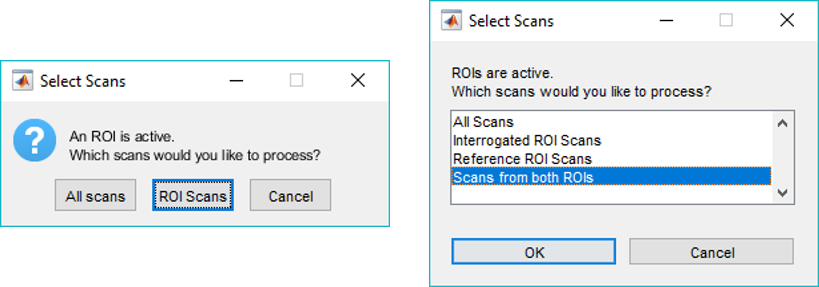
Figure 93: Active ROI dialogs for a single ROI (left) and two ROIs (right).
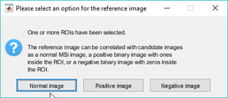
Figure 94: Normal or binary reference image dialog.
If scans from ROIs are selected a second dialog gives the user the option to make the reference image positive or negative, that is, 1’s inside the ROI and 0’s outside of it or the other way around. The dialog is not shown if All scans is selected. This dialog is shown in Figure 94.
With the options selected in Figure 90 and the parameters shown in either in Figure 91 or Figure 92, “virtual” images would be generated in memory, correlated with the reference for each set of SSIM parameters and scored. The output folder would be filled with image files for the highest ranked results (user-defined – see Figure 90). The top 100 m/z values and scores would be saved in a text file in the same folder. If you want to save all of the scores, enter Inf or All in the Scores to Save data box (Figure 90). Before ranking over 280,000 images it is advisable to use peak picking to generate a smaller list of m/z candidates to see how long this process takes with your data. The SSIM algorithm is very fast, scoring a pair of images with 1 million elements each in less than 120 milliseconds on an ordinary laptop. However, generating the internal data for each candidate image will consume significantly more time.
A progress bar is displayed during the correlation process. If it is closed, the user is prompted to confirm terminating the image correlation or to continue. Continuing will skip the remaining candidate images and proceed with sorting the scores obtained so far and saving graphic image files. Another progress bar is displayed while the files are generated. You can open the folder where they are being saved to see a preview of your images. This process can also be stopped early by closing the progress bar again.
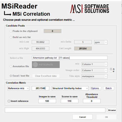
Figure 95: The MSiCorrelation tool using a .txt file as the input. Click browse to select a file for the output folder for the images to be generated.
MSiCorrelation uses the current MSiReader parameters when generating images (e.g., MMA, colorscale). You may lock the heatmap scale in the MS Navigation pane so that all images are generated on the same scale. Next, the user has 4 choices of candidate m/z values: clipboard contents; build an m/z list, choose an annotation file or select Excel or text file to upload a series of m/z values for the correlation analysis. In this example, a .txt file with a list of m/z values that the user would like to determine if they correlate with the reference m/z value. The reference m/z value that was chosen is 283.1540 as shown in Figure 95. If the user selects none – this is batch image generation; if the user selects reference m/z, this will be a MSI image of that m/z value and lastly, external data, this selection allows you to use an optical overlay for correlation.
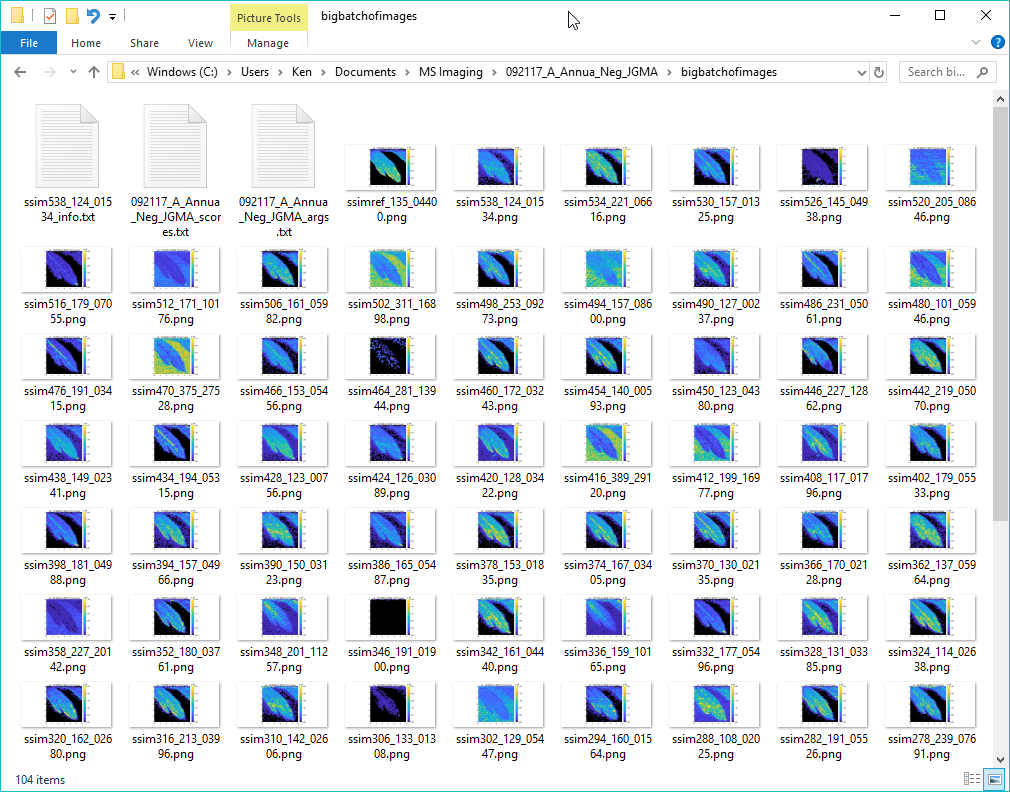
Figure 96: A folder of images created by MSiCorrelation.
An example of a folder of ranked images is shown in Figure 96. The image files are named using the correlation method, the rank and the m/z value for easy identification and sorting. The reference image is also saved in this folder.
Two or three text files are also saved using the data set name. A <name>_info.txt file containing current MSiReader and MSiCorrelation settings is shown in Figure 97. If SSIM was the selected method another file <name>_args.txt is written. Lastly, the scores are saved. An example is shown in Figure 98 with the m/z values and their score. The third column is the index (i.e., line number or row) into the SSIM parameter file used to obtain that score.
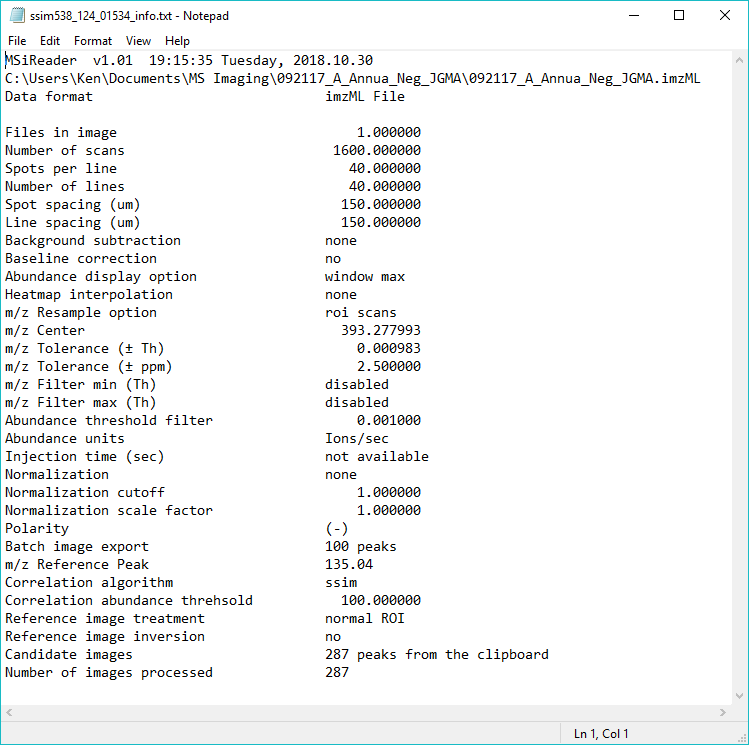
Figure 97: Text information file with data set and correlation parameters.
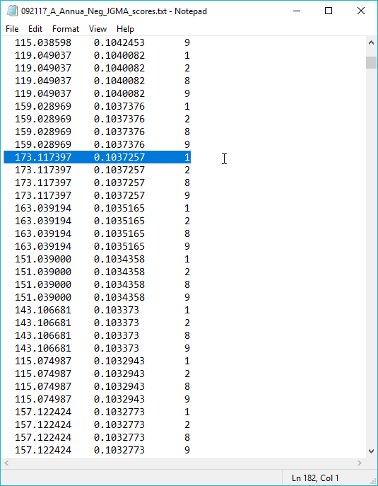
Figure 98: Correlation scores files showing m/z values, their score and the row of the corresponding parameter set that was used to obtain that ranking. The highlighted text is the 182nd highest ranked candidate on line 182 of the file.
7.6.4 ROI Functions
Restoring a previous ROI or defining an ROI (single pixel/voxel), line, or polygon can be done using these menu items or their associated ICONS in the toolbar.  Restore a previously saved ROI. Select a single scan ROI using the cursor tool. Use this selection in the pull-down to select a single pixel (or voxel) in the heatmap. The user can drag this around using the mouse. Once a selected pixel of interest is decided upon, the user can right click and a sub-menu comes up allowing one to export the coordinates, change the color of the cursor, or plot the mass spectrum for the collected (or filtered) m/z range. When viewing the mass spectrum, there is a new toolbar at the top. These allow one to save the plot as a MATLAB .fig file, or print the spectrum. The next band of icons in the toolbar allows you to select a peak in the mass spectrum and update the heatmap for that specific m/z. You can also copy details to the clipboard for the selected peak. Once you select a pixel in the main GUI, right click on pixel and select “Plot m/z spectrum”. Now the mass spectrum is shown and the user can move the cursors to different peaks in the mass spectrum and the heatmap(s) will auto update. In this way, a user can quickly look for spatial distributions and identify background ions.
If the user wishes to select all pixels for data export, the user can load the data and go directly to MSiExport. Since no ROI was selected, it will export all the pixels/wells. This is particularly useful for the BioPharma mode so users do not have to select a polygon tool and then say “All Scans” when opening up the MSiExport tool.
Select an ROI using the segmented line drawing tool. Click this selection in the pull-down to select a line of any length or direction through the heatmap. Upon doing so, the length of the line will be shown on the top left of the heatmap. If you right click on the line in the image, you will be able to: 1) export the line ROI details; 2) set line color; 3) plot the ion abundance as a function of distance along the ROI line; and 4) select plot type (stem, stairs, or line).
Select an ROI using the polygon drawing tool. If you right click on the polygon in the image, you will be able to: 1) export the line ROI details; 2) make the ROI a rectangle; 3) select all pixels for the ROI; 4) create a binary mask for the ROI; and 5) set line color. The user can generate a binary mask using the polygon drawing tool or the interrogated and reference regions; the binary mask is simply a matrix of 0’s and 1’s applied to a given dataset.
 Select interrogated and reference ROIs using the polygon tool. This is done to compare two regions of interest using, for example, MSiPeakfinder (§7.7.1).
The user can apply a binary mask that they created after selecting a ROI using the polygon tool or the interrogated and reference ROI tool. If the user selects from the Annotations menu then ROI then “Apply binary ROI mask to heatmap” but has not selected one or two ROI’s, the matrix applied is all 1’s (no change in heat map). If one or two ROI’s are defined, the user can right click on either ROI and a menu will allow you to create a binary mask and include interrogated ROI, reference ROI or all scan in both ROI’s. If they are overlapping regions, you will have an additional option. To turn ON or OFF the binary mask, the user simply selects this option in the drop-down menu (toggle). One use of this function might be to focus on a cancer ROI and a healthy ROI and thus, visually remove the other regions of the tissue and the image saved.
7.6.5 MSiCorrelation and Batch Processing
The MSiCorrelation tool provides a convenient way to generate and order batch images for the m/z values in a METASPACE annotation file, an Excel file, the clipboard or for a uniformly spaced m/z list. The image files can be named so they appear in a desirable order in the output folder. This can be by m/z value, according to another column of the same input file, or by their correlation rank. For correlation ranking, the images are generated virtually and compared with the reference image using the selected algorithm. Then the specified number of top ranked images are saved in the output folder. The MSiCorrelation tool user interface is shown in Figure 95.
Peak Source and Image Order
The source of m/z values can be the clipboard contents, a METASPACE annotation file, an Excel worksheet, a text file, or a list with uniform spacing can be generated by the tool. In the case of an Excel workbook, the user is prompted to select a worksheet. The m/z and Image order pull-down menus in the Candidate Peaks panel are automatically populated with the column headings from the selected worksheet, a text file, or a METASPACE .csv format annotation file.
Only columns containing numeric data will be added to the m/z column list. The image order column can be numeric or text. If column headings are not present the strings “Column A”, “Column B”, etc. are used for Excel files and “Column 1”, “Column 2”, etc., for text files. Whenever a new column is selected the number of m/z values within the range of the current data set is displayed next to the file name in square brackets. There must be at least one value for the OK button to be enabled.
The method for specifying exported and batch heatmap plot titles is defined as follows. There are six title styles and ten title elements. The preferences INI file (§5) variables ExportFigTitleStyle and BatchFigTitleStyle can be any of the style names or a custom style can be specified mnemonically. This allows the elements to be used in any order. The number of elements on each line of the title are controlled by using the semicolon character to indicate a line break.
The allowed title elements and their meaning are:
mz m/z value
tolerance tolerance in ppm units
mzwindow tolerance in Th units
formula molecular formula METASPACE annotation only
adduct adduct formula METASPACE annotation only
normalization normalization option (none, TIC, max, ...)
pixelation m/z window treatment (max, sum, mean)
dimensions columns and rows in the data set
interpolation heatmap interpolation algorithm and order
comment user comment
filename data set name
Using these elements, the predefined styles are:
none no title
short mz
batch mz tolerance
trim comment; mz tolerance
metaspace formula adduct; mz tolerance
full mz tolerance mzwindow; formula adduct; normalization; pixelation; dimensions; interpolation; comment; filename
The file generated for each image is named using a prefix containing its sequence number in the sorted list followed by the m/z value of the image. For example, “seq032_369_3516.png”, for the 32nd image with m/z 369.3516. This gives the user a way to order the images in the output folder other than by m/z value. The up triangle and down triangle radio buttons to the right of the Image order pull-down menu are used to select the sorting direction. If all of the values in the ordering column contain numbers, a numeric sort is used. Otherwise, sorting is alphabetically. For example, the molecular formula C18H36O2 occurs before C6H8O7 in ascending alphabetic order. In both cases, the sorting algorithm is stable, i.e., the relative order of equal values is preserved.
An example of a folder of batch images is shown in Figure 99. The images are ordered according to decreasing MSM value for a METASPACE annotation file.
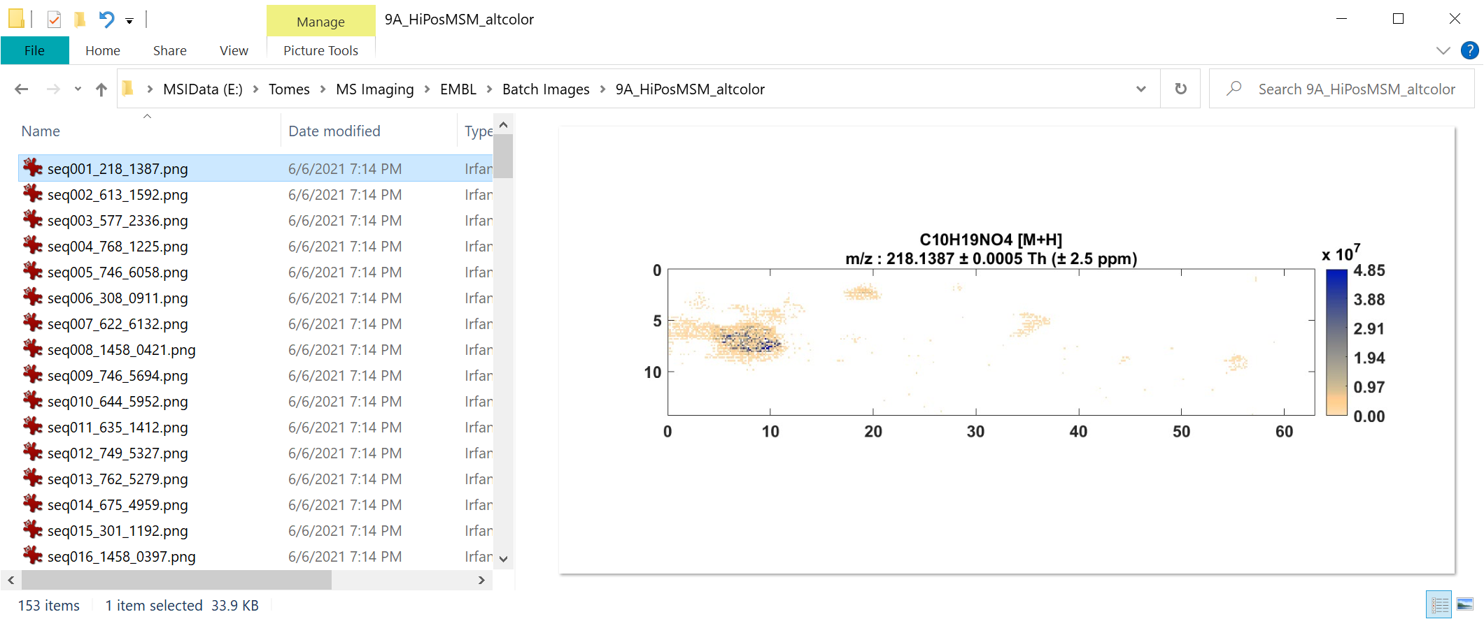
Figure 99: A folder of batch images ordered by MSM value.
In addition to the image files, two text files are saved in the same folder. Figure 100 shows the contents of the “Info” file which contains details of the MSiReader settings and MSiCorrelation selections (upper), and the list of m/z values and image order values for each image in the folder (lower). If batch image creation is stopped by clicking the MSiReader STOP button before completion, the peaks list file will have data only for the images that were generated.
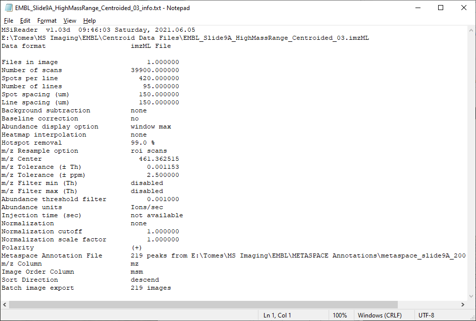
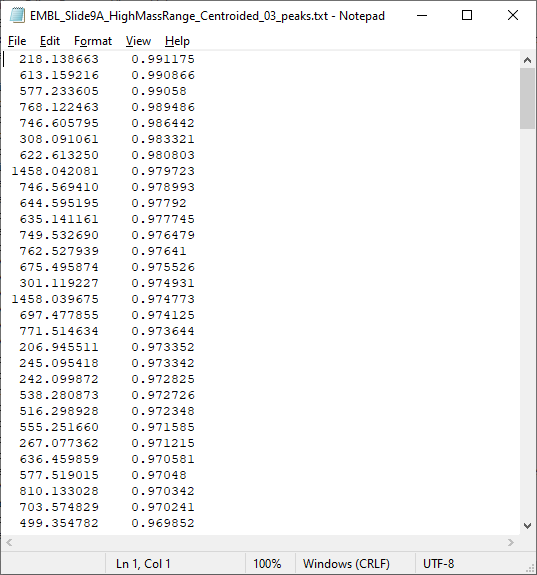
Figure 100: Information file with MSiReader and MSiCorrelation parameters (top) and peaks list file (bottom) for the images folder shown in Figure 99.
METASPACE Annotation Format
The MSiReaderPrefs.INI file (§5) contains variables that define the meaning of the columns in a METASPACE annotation file. This provides a means to accommodate future changes to the format and for the user to enhance the format with additional columns of information or create an entirely new format of annotation file. These variables are defined in Table 5.
Table 5. METASPACE variables in the MSiReader preferences INI file (§5).
Variable | Default Value | Meaning |
MetaspaceHeaderRow | 3 | Row containing column heading character strings. |
MetaspaceFirstRow | 4 | The first row containing data values. |
MetaspaceMassSelectionColumns | 6 | Columns used to create the m/z pull-down menu. |
MetaspaceRankSelectionColumns | 4 5 6 7 8 9 10 11 | Columns used to create the Image order pull-down menu. |
MetaspaceMassSelectionDefault | 6 | Default m/z selection column. |
MetaspaceRankSelectionDefault | 6 | Default Image order selection column. |
MetaspaceMoleFormColumn | 4 | Column containing molecular formulas. |
MetaspaceAdductColumn | 5 | Column containing adduct names. |
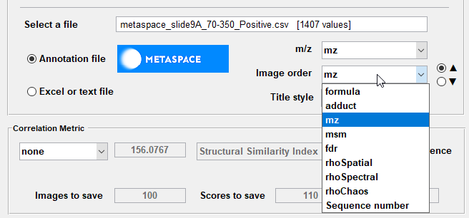
Figure 101: Image order selection for a METASPACE annotation file.
After loading a METASPACE annotation file the Image order pull-down menu appears as shown in Figure 101. Note that an additional item, Sequence number, is always added to the end of the list. If it is selected the m/z values are not sorted and the images are assigned sequence numbers according to their order in the CSV file. Sequence number is also added to the menu when an Excel or text file is selected.
The right-click context menu for the Annotation file and Excel or text file radio buttons is used to clear loaded data so a new file can be selected as the m/z peak source as shown in Figure 102.
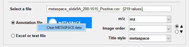
Figure 102: Clearing a loaded METASPACE annotation file (right click on Annotation file). If using Excel or a text file, right click on there will clear those annotation files.
Batch Image Titles
Batch image heatmap plot titles can be formed from the ten elements shown in Table 6.
Table 6. Batch image title elements.
Name | Meaning |
mz | The m/z value for the heatmap. |
tolerance | The tolerance window in Th and ppm units. |
formula | The molecular formula. |
adduct | The adduct formula. |
normalization | The current normalization option: TIC, max, mean, median, etc. |
pixelation | The abundance treatment for each pixel: max, mean, or sum. |
dimensions | The image dimension in pixels. |
interpolation | The heatmap interpolation algorithm and order. |
comment | The user comment value. |
filename | The name of the loaded data set. |
There are six predefined formats for the titles of batch heatmap images: none, short, batch, trim, metaspace, and full. These styles are defined using these elements from Table 7 and the semicolon character as shown in Table 7; a semicolon starts a new line in the title.
Table 7. Batch title styles created using the title elements.
Name | Title Style |
none | no title |
short | mz |
trim | mz tolerance |
batch | comment; mz tolerance |
metaspace | formula adduct; mz tolerance |
full | mz tolerance; formula adduct; normalization; pixelation; dimensions; interpolation; comment; filename |
In the preferences INI file (§5) the BatchFigTitleStyle variable can be set to any of the style names or a custom style can be created using the element names from Table 7 and the semicolon character. When each image is created the actual values are substituted into the title style string in the order specified. Blank lines are omitted from the plot title (e.g., when no user comment is defined).
Figure 103 shows the title style pull-down menu. The additional style, custom, is always the last selection in the menu and refers to the style given for the BatchFigTitleStyle variable in the INI file (§5), whether or not it is the one of the six named styles in Table 7.
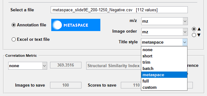
Figure 103: Title style selection.
For example, if the MSiReaderPrefs.INI file (§5) has,
BatchFigTitleStyle = mz tolerance; formula adduct; filename
and custom is selected from the pull-down menu, a three-line title will be created similar to the one shown in Figure 104.
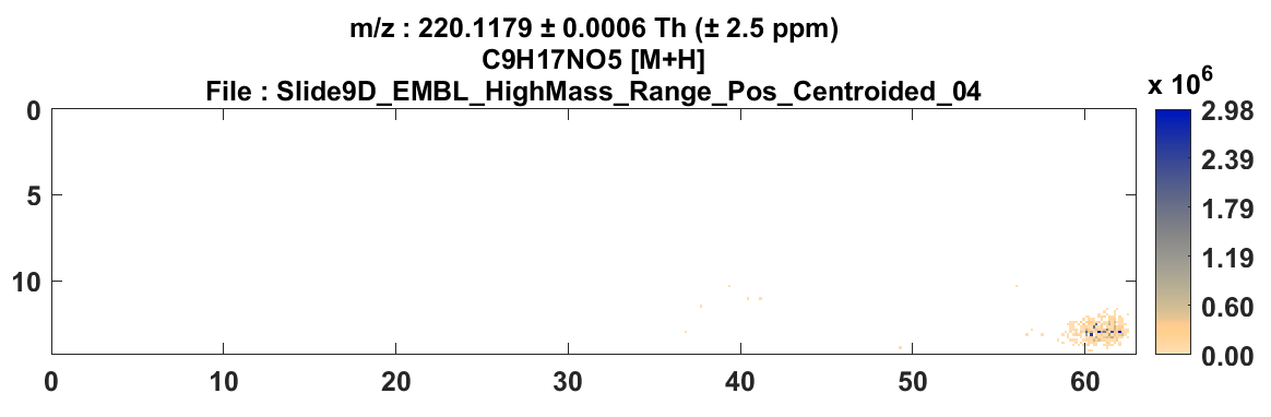
Figure 104: Example of the custom title style with m/z, tolerance, molecular formula, adduct, and file name.
However, if the metaspace style is selected from the pull-down menu, the same plot would have the title shown in Figure 105.
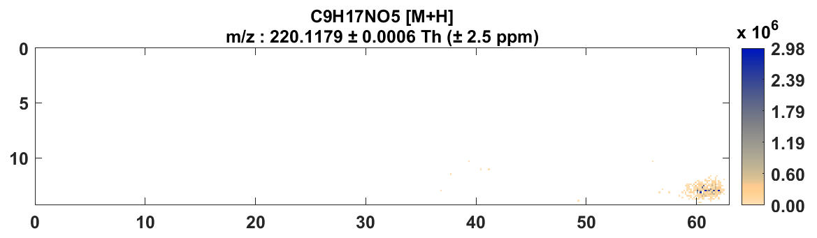
Figure 105: An example of the metaspace title style with molecular formula, adduct, m/z, and tolerance.
7.6.6 Data Export
7.6.6.1 MSi Spectrum (generate mass spectrum)

Using the above icons in the toolbar, the user can load a previously saved ROI, select a single scan, a region of interest or the entire data set and export useful information such as
Averaged spectrum. See below.
Raw individual mass spectra. See below.
Abundance values for single or multiple m/z values.
Spectral abundance binned over an m/z range.
The user must first select the scan(s) in the current image that are to be processed. The default tool to select a region is polygon where the region is chosen by selecting multiple points to form a closed area. Double click to connect the last point to the first and close the polygon. At any time, the user can right-click and force the region to become a rectangle. Points from the polygon region can be deleted, dragged around or new points added (hold down the “A” key and click on any line segment in the polygon) to modify the shape. A single scan region can be created by double clicking once without drawing a line. The default selection tool can be changed to freehand (region is drawn over tissue with mouse cursor) or rectangle in the preferences INI file (§5). Freehand ROIs are converted to polygons when the region is closed. The image zoom and pan tools are not reset during ROI selection so that you can zoom in to more accurately select a small region. Most of the other tools also remain enabled allowing you to change the m/z value, window units, normalization, interpolation, heatmap color scale and colormap.
Load a previously saved ROI. Pressing this button will launch a file selection dialog for the user to choose a .mat file containing a previously saved ROI. Saving an ROI is described in §2.4.3. The user will be warned if the ROI was originally drawn on a different file or if the present dimensions and scaling do not match the saved information, but the user will not be prevented from loading it. If the file contains two ROIs, the user will be prompted to select either one or both of them. The ROI(s) will be drawn at the saved X and Y locations on the current heatmap. The toolbar icons for MSiSpectrum, MSiPeakfinder, and MSiQuantification will be enabled if appropriate and the icon used to draw the original ROI will be “toggled”.
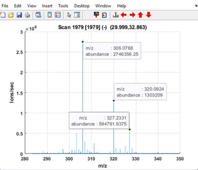
Figure 106: Spectrum plot for a single scan. The title contains the scan number, polarity and location in the image. The data cursor tool has been customized by MSiReader to show the m/z and abundance value for the selected peaks.
Use cursor to select a single scan. A cursor will appear on the heatmap and can be dragged to any desired location. Note that any interpolation scheme will be automatically removed after user has pressed this button. A mass spectrum like the one shown in Figure 106 can be enabled for the scan under the cursor by right-clicking the selected scan. The plot will update automatically as the cursor tool is moved. The abundance and polarity for the scan at the current m/z is displayed above the heatmap plot and updates automatically as either the cursor is moved, or the m/z value is changed.
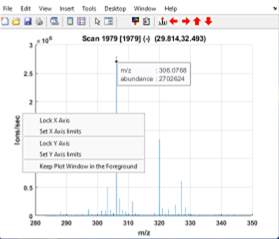
Figure 107: Context menu selections for spectrum plot options.
The plot also has a context menu with five items. The last one keeps the plot in the foreground and the others can be used to set or lock the horizontal and vertical axes (Figure 107). Two icons have been added to the spectrum plot toolbar. Clicking on the icon updates the MSiReader heatmap with a data cursor m/z value. If there are multiple data cursors the user is prompted to select one. The selected m/z value is also added to the m/z history list. The icon appends all of the data cursor m/z values to the clipboard.
Use cursor to select the scans along a segmented line. After pressing this toggle button, the user can draw a segmented line on the heatmap to define the ROI. The scans that the line intersects are in the ROI. Note that any interpolation scheme will be automatically removed after the user has pressed this button. Like the polygon tool, data points on the line can be moved or added after the ROI is drawn. The line length, abundance mean, standard deviation, minimum and maximum values are displayed above the heatmap plot and update automatically as the ROI is moved or the m/z value is changed. An abundance plot of the scans along this ROI like the one shown in Figure 108 can be enabled by right-clicking on the line. As the line is moved or edited or the m/z value is changed the plot automatically updates.
The plot also has a context menu (right mouse click on the line segment) with five items: Export slice line location information, set color, delete vertex, plot slice line abundance, and select slice plot style (with sub-menu).
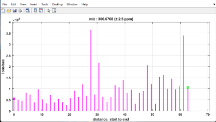
Figure 108: Abundance plot along a segmented line. Locations of the connecting points for the line segments are marked with a black x (if not just a single line), the magenta square and the green circle mark the beginning and end of the ROI, respectively.
Use ROI tool to select a region of interest containing multiple scans. After pressing this toggle button, the user can draw any shape on the heatmap to draw an ROI. Note that any interpolation scheme will be automatically removed after user has pressed this button. The area, and abundance mean, standard deviation, minimum and maximum values are displayed above the heatmap plot and update automatically as the ROI is moved or the m/z value is changed.
Select all scans from the image. After drawing the ROI (even a single scan ROI), the right-click context menu for the ROI object can be used to expand the ROI to include all scans in the image. This option is particularly useful for users who want to build heatmaps by combining the abundance value of multiple m/z’s (e.g., sum, ratio). The user can export abundances for multiple m/z’s, process them in Excel and load the result as a custom heatmap. The area and abundance mean, standard deviation, minimum and maximum values are displayed above the heatmap plot and update automatically if the m/z value is changed.
Once the scan or region of interest has been successfully defined, the toolbar icons allowing the user to export spectrum data or heatmap abundances for those selected scans are enabled. These features are described here.
 Export and view mass spectrum data for a cursor or ROI. Upon pressing the icon (or drop down menu under Annotations then Data export then Generate mass spectrum) the MSiSpectrum sub-GUI is launched and several options for data processing and spectrum export will be offered to the user (see Figure 109). The user can also choose to extract the data and a centroided peak list to Excel. Options for centroid calculation can be selected in the GUI (minimum abundance threshold, centroid algorithm, etc.). When centroiding data for an ROI or building an average spectrum the m/z values from the scans must be resampled to a common set of values. If the data set was loaded with scans having both (+) and (-) polarity, a button group is enabled to select a polarity option, including both polarities.
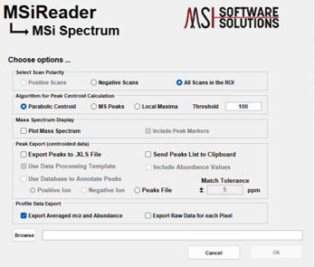
Figure 109: MSiSpectrum GUI to export a mass spectrum.
Users can also export individual unprocessed profile data for each of the selected scans to an Excel spreadsheet. Note that this operation may take a long time for a large dataset. If the dataset is too large to be exported to Excel, or Excel is not installed an alternate text format is used. A preference .INI file entry (§5) is also available to select text instead of Excel export. Note that unprocessed scan export to a text file can be up to 300 times faster than to an Excel workbook.
The figure toolbar contains navigation tools (zoom, pan) as well as a data cursor tool  that shows the m/z and abundance at a selected point on the plot. As shown in the Figure 110, multiple data cursors can be added to customize a plot. Magenta marker lines or dots are added as well. The markers can be temporarily hidden by clicking on Peak Markers in the legend. The markers (dots or lines) will be hidden until Peak Markers is clicked again. Similarly, spectrum visibility can be toggled by clicking on ROI Spectrum in the legend. The preferences INI file (§5) variable MaxMarkerstoView sets the marker dialog threshold and SpectrumPlotStyle and SpectumPlotMarkerStyle define the line style (line, stem or stairs) and the marker style (point or line).
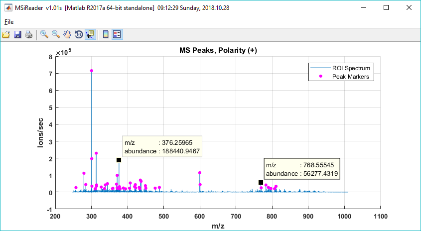
Figure 110: Plotting a mass spectrum in MSiReader.
Exporting ROI location information
After selecting an ROI, the location and scan number of all scans in the ROI can be exported into a text file simply by right-clicking on the ROI and selecting Export ROI Location Info. The text file generated will contain 4 columns:
Column 1: Scan number from the original file (assuming meandering, fly back raster pattern)
Column 2: X location on image (column number)
Column 3: Y location on image (row number)
Column 4: Z location on image. Note that if a non-square ROI is exported, the smallest enclosing rectangle will be exported and the scans that are were not in the ROI will be marked as –Z (e.g. -1).
Note that this file format can be used as a location file when loading mzXML and imzML files. Only the scans in the ROI will be loaded!
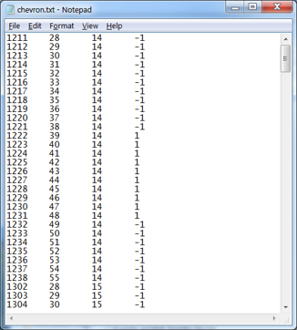
Figure 111: Example of output file generated by ROI export tool.
For a tiled image mosaic of a folder of imzML or mzXML files, the ROI location file will have two more columns containing the file number and original scan number of each scan in its file. The first three columns are always the scan number and X,Y location of the scan in the displayed image. An example is shown in Figure 111.
In addition to the text file described above, a .mat file using the same name is created containing the location information, the file name, and the number of columns and rows. This file can be used to load the ROI into a future MSiReader session in the same location where it was originally drawn.
7.6.6.2 MSi Export (export abundance data)
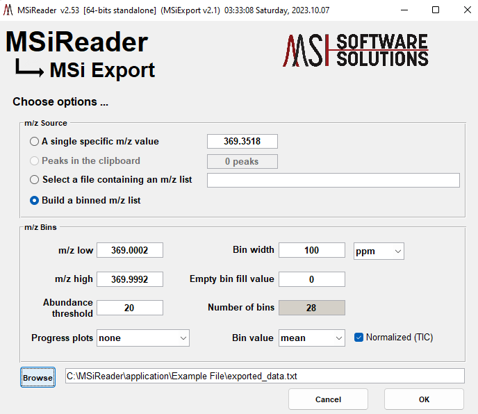
Figure 112: GUI for MSiExport tool.
This icon launches the MSiExport tool which allows the user to export raw or normalized abundance values for each scan in an ROI or to bin the abundance values into a specified m/z range. First the user selects a scan, an ROI, or all of the image scans using the icons in the toolbar. Then after selecting the icon in the toolbar or from drop-down menu, select “export abundance data” under Annotations and then Data Export - the MSiExport GUI shown in Figure 112 is launched.
Four options are given for the m/z value(s) to export: a single value, the values in the clipboard, a list of m/z values in a file (*.xlsx, *.txt or *.csv), or a uniformly spaced list (by Th or ppm). For the first three options the raw scan data can be exported to the Excel format shown in Figure 113.
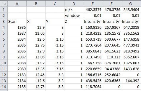
Figure 113: Format of abundance data extracted from an ROI to an Excel file.
If Excel is not installed, the amount of data is too large, or the preferences INI (§5) variable ExportPixelsToText is set to true, two text files are created instead. One contains the MSiReader settings normally sent to the Info worksheet (e.g., date and time, file name, number of scans, window and filtering options, etc.) and the other has the raw scan data. Examples of these files are shown in Figure 114. All abundance values are calculated using the current m/z window and abundance calculation method. Normalization is also applied if any method has been selected. If the loaded data is from a folder of imzML or mzXML files, two columns of data are added to the Excel file shown in Figure 113, the file index number and the local scan number from that file. For the text format, two
additional rows are added to the file shown in Figure 114 with this information. The index numbers are simply the tile locations in row-major number. Additionally, a worksheet is added to the Excel file with the tiling pattern and a list of the file names.
If you selected a file of m/z values as the source, you can load another file by right-clicking on the Select a file containing an m/z list radio button text to launch the selection dialog again.
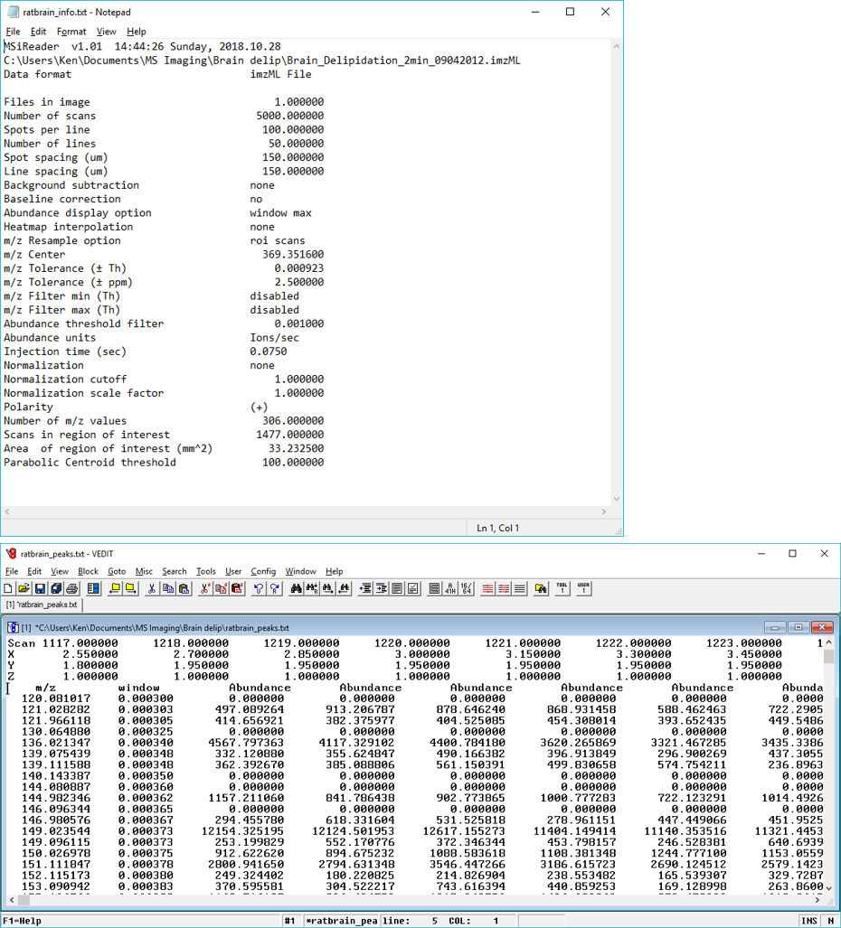
Figure 114: Scan abundance data exported from an ROI to two text files. Above is the header information showing MSiReader parameters and settings and below is a portion of the abundance matrix for the selected scans.
Binned scan data export
Selecting Build an m/z list and bin the pixels in the ROI in the MSiExport tool allows the user to export spectral data for the selected ROI that has been binned over a uniformly spaced m/z range. This can be done using unnormalized data or normalized data – if the end user wishes to normalize the data, this selection must be done in the main MSiReader GUI first prior to exporting the binned data. This facilitates external processing of the ROI with a multivariate analysis tool such as MSiPCA (§7.8.2) or t-SNE (§7.8.3). For this selection the data set may be very large and sparse and thus is always exported to a text file. A *.csv file can also be generated for use in MSiReader (not recommended) or for use in other data analysis programs. The m/z Bins pane in Figure 112 is used to select the binning options. Note that in this case, the data was normalized to the TIC and that is is shown on the bottom right of the GUI so the user knows that the data is normalized and how it was normalized. Their meaning and default values are given in Table 8.
Table 8. Binning options.
Bin width (m/z) | full width of each bin |
Bin units (ppm or Th) | units of the bin width value |
m/z Low | smallest m/z value, lower edge of the 1st bin |
m/z High | largest m/z value, upper edge of the last bin |
Empty Bin Fill Value | the value to use for an empty bin |
Abundance Threshold | abundance filter, data points with abundance lower than this value are excluded |
Bin Result | selects mean, sum or max as the value saved in each bin |
Plots | no plots, one plot updated in real-time as the bins are created, or a separate plot for each bin |
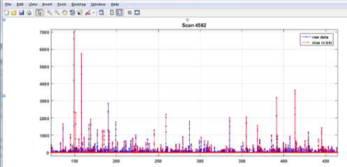
Figure 115: Plot showing original and binned spectrum for a scan.
The initial values for the bin range are the smallest and largest m/z values in any of the selected scans. The abundance threshold can be used to filter out low abundance noise by including only those peaks above the entered threshold. The empty bin fill value can be any numeric value desired, including Inf (positive infinity), -Inf (negative infinity) and NaN (not-a-number). Each bin in the output file will contain either the mean abundance, sum of abundances or maximum abundance of the m/z values that fall in that bin. Finally, the plot option allows the user to observe the binning progress as it is applied to each scan on a continuously updated plot similar to the one in Figure 115. This is useful for exploring the tradeoff between the filter threshold and the bin width. Do not select the Separate Plots option if the ROI has a large number of scans; this will likely cause your computer to lock up.
After the options are selected the user is prompted for a name and location to save the binned data. The file is written in a text format shown in Figure 116 or can be output as a *.csv file. The first 36 lines of the text file contain the name of the data set, MSiReader options and parameters and the binning options, next is a vector with the m/z values for the center of each bin. As shown in the figure, each row of the binned abundance matrix corresponds to a scan from the ROI where the first 6 columns give the spatial location of that scan. For this example, the data was a folder of imzML files so the file number and local scan number for each scan are also given. The remaining columns contain the composite abundance values (mean, sum or max) for each bin.
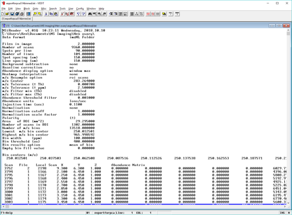
Figure 116: Example of the binned data text file format.
The exported text file may be very large and unsuitable for opening with Notepad. The text format was chosen to facilitate input for further analysis, for example MSiPCA. Two Matlab functions are included in the MSiReader installation to process a binned data export file: getmsibindatainfo and loadmsibindata. The first function can be used to query the file without opening it with a text editor and before reading it into a program. This is useful for assessing the resource requirements of a very large data set to determine if you have sufficient memory to process it or if you should export it again with a larger bin size (and thus fewer bins) or a higher filter threshold. The second function, loadmsibindata, loads the data set into a Matlab matrix and returns the center m/z for each bin, the list of scans in the ROI and the same information structure returned by getmisbindatainfo. The binned abundance matrix can optionally be returned as a Matlab sparse matrix instead of a full rank matrix containing many zero entries. Both functions have help text that can be viewed by typing help getmsibindatainfo and help loadmsibindata in the Matlab command window.
7.7.1 Relative – MSi Peakfinder
For a video tutorial on how to use MSiPeakfinder, click HERE.
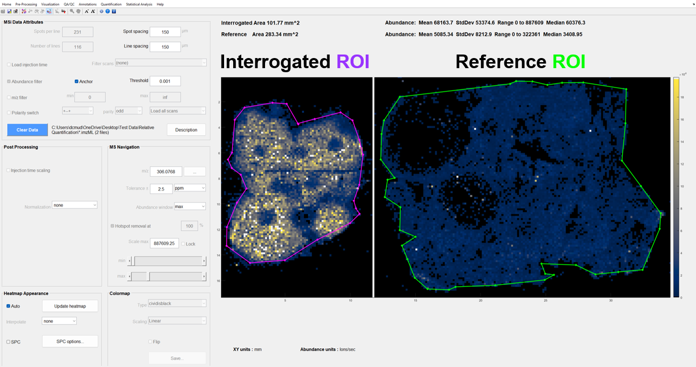
Figure 117: Automatic peak detection process using MSi Peakfinder. Start this process by selecting a reference and interrogated ROI.
MSiReader implements a peak picking strategy to identify ions in a sample that are more abundant in a user defined interrogated ROI as compared to a reference ROI as shown in Figure 117. Peaks are detected by comparing the average abundance of each m/z value and its occurrence over both user defined ROIs. Criteria used for detection are user defined and can be easily modified within the interface. A mass spectrum plot showing the superimposed averaged signal for both the interrogated and the reference ROIs is optionally generated (Figure 118 and Figure 119) and can be used to browse through the peak list. The extracted peak list can also be sent to the clipboard or saved into an Excel workbook.
The process begins when the user presses the  toolbar icon to select the interrogated and reference ROIs using the polygon drawing tool and proceeds as follows. Alternatively, the toolbar icon may be used to select previously saved interrogated and references ROIs.
Any interpolation scheme will be removed so that each pixel corresponds to a single mass spectrum.
The user draws the interrogated and reference ROIs or loads a saved ROI .mat file containing both the interrogated and reference ROIs.
When the user selects Relative MSi Peakfinder under the Quantification menu, the MSiPeakfinder GUI is called and the user selects parameters for the peak finding algorithm as shown in Figure 118.
After clicking the OK button, all spectra in the interrogated ROI are averaged and a peak list is generated. A progress bar is shown at the bottom to give the user an indication of the length of time remaining for processing.
Then all spectra in the reference ROI are averaged and a second peak list is generated. This is done automatically. The progress bar shown at the bottom starts over for the reference ROI to give the user an indication of the length of time remaining for processing. Steps 4 and 5 require a lot of data processing so please be patient.
The resulting peak list is copied to an Excel worksheet that can be used as an input file for the correlation and batch processing of images. (§7.6.5) If the Mass Excess template file is selected, lipid plots are automatically generated when the peaks are inserted into the worksheet.
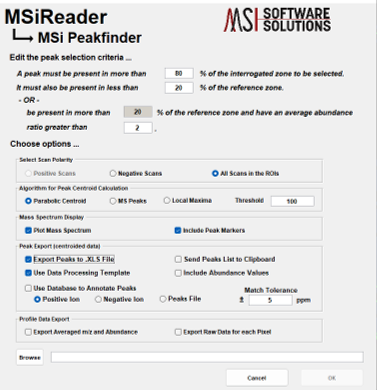
Figure 118: MSiPeakfinder GUI used to select peak picking parameters and options.
The interrogated and reference ROIs have context menus to export location information (i.e., the scan numbers and X, Y location of each scan), change the line color, convert the ROI into a rectangle and to swap the reference and interrogated ROIs. This latter feature can be used to easily carry out a two-way comparison between ROIs without having to move or redraw them. If a folder of imzML or mzXML files were loaded, the ROIs can be anywhere in the image mosaic.
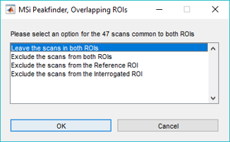
Figure 119: Overlapping ROI action dialog.
In the case of overlapping interrogated and reference ROIs there are several ways to treat the scans in both regions when applying the peak picking algorithm. The user is prompted to select an option as shown in Figure 119.
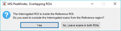
Figure 120: Dialog for the special case of an interrogated ROI that is inside the reference ROI.
In the case of one ROI being completely enclosed inside the other (e.g., the interrogated ROI is inside the reference ROI) only two of the choices make sense and the dialog in Figure 120 is shown. If the reference ROI is inside the interrogated ROI a similar dialog is displayed. Coupled with the ability to expand an ROI to be all scans, this is a convenient way to compare all background scans (reference ROI) with tissue scans (interrogated ROI).
Note that the tolerance for peak comparison between the interrogated and reference ROIs is specified by the user defined m/z window when the peak finding feature is launched. If the m/z window units are chosen by the user to be parts-per-million (ppm) in the MS Navigation panel, a ppm m/z window will also be used when peaks are compared. Information about necessary resampling steps when averaging data as well as the centroid calculation are given below.
Resampling
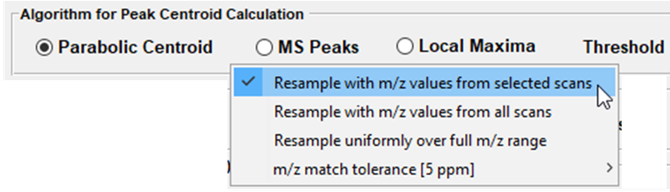
Figure 121: Context menu for selecting an m/z resampling algorithm.
Some of the imaging data may be processed by the instrument vendor software or the format converters to reduce the file size (e.g., zeros are omitted), and therefore the spacing between the data points on the m/z scale and the total number of data points are not the same for every scan. Prior to averaging spectra over a certain ROI, each individual spectrum of the ROI must be resampled to a common set of m/z values. This means that omitted zero values may have to be added and some data points will be interpolated. Resampling is only done when peak picking is performed or when spectra are averaged. One of three m/z resample options can be selected with a context-menu (right mouse click) for the Algorithm for Peak Centroid Calculation Panel in either MSiSpectrum or MSiPeakfinder as shown in Figure 121.
Option 1: Resample to all existing data points on the m/z scale found in all the spectra in the ROI (default option).
Option 2: Resample to all existing data points on the m/z scale for all the spectra in the image (no matter where the ROI is).
Option 3: Resample all scans uniformly over the entire m/z range, regardless of the presence of a signal for a particular m/z in any of the scans. If the m/z data points are systematically different from spectrum to spectrum it is preferable to use this Option instead of Option 1 or 2, either of which may generate an extremely large number of m/z data points for this case.
The implementation of the resampling options in MSiReader improves performance. The new algorithm for merging m/z vectors from the scans in an ROI can be as much as 100 times faster. Previously, as the m/z values from separate scans were combined into a single vector only exact duplicates were removed. Now a tolerance for this test is used. The tolerance can be expressed as an absolute minimum difference in Th units or as a ppm value. The tolerance value and units can be changed using the final context menu item, m/z match tolerance [5 ppm], in Figure 121. The preference INI file (§5) variable mzResampleOption can be used to select a default resampling algorithm. The tolerance value defaults to the current MSiReader Navigation panel settings when MSiSpectrum or MSiPeakfinder is launched. The upper limit on the size of the resampled m/z vector can be set with the mzResampleMaxPts variable in the preferences INI file (§5). The default value is 1e7. If the number of m/z values needed for resampling exceeds this value, the user is prompted to confirm switching to Option 3 to resample uniformly or to abort the peak picking operation.
Algorithm for centroid calculation
Three different algorithms can be used to extract a peak list from the spectrum data (selection was made in MSiPeakfinder GUI shown in Figure 118). The algorithms use different approaches to calculate the centroid from the mass spectrum data. The first option is to use a Parabolic Centroid Algorithm. This algorithm was proposed by Comisarow and Marshall in their early work interpreting FTMS spectra20,21. For each local maximum in a mass spectrum, the centroid location will be the calculated m/z of the apex of a parabola fit to that local maximum and the 2 adjacent points (see Figure 122). The centroid locations calculated with this method are nearly identical (within a fraction of ppm) to those calculated by using instrument manufacturer software.
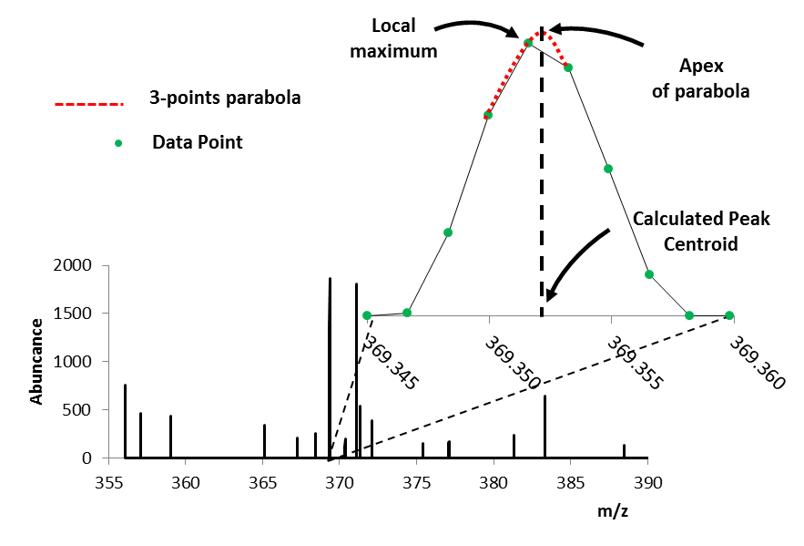
Figure 122: Calculated peak location using Parabolic Centroid Algorithm.
The second algorithm uses mspeaks function to calculate peak centroid locations.
The third algorithm is to select the m/z with the maximum abundance value in each data window as a peak. This is of course the fastest of the three algorithms and ensures that selected peaks have m/z values and abundances that are identical to data points in the original scan data.
The basic settings and options of this function can be easily changed using the preferences INI file (§5). Also note that using mspeaks may increase computation time significantly.
IMPORTANT: The first two centroid algorithms may produce unexpected results if the input file is not an actual mass spectrum but a peak list (preprocessed centroid data).
Saving Results in MSi Spectrum and MSi Peakfinder
The user is given the option to export data in Excel or text format from both the MSiSpectrum GUI and the MSiPeakfinder GUI. Excel format is selected by default; however, a text format will be used if Excel is not installed, the size of the data to be exported exceeds the limits of Excel or the INI preferences variable ExportToExcel is set to false. Depending on the options selected on the GUI, here is a description of the worksheets or text files that will be generated:
Info: Contains information about the version of MSiReader used to export the data, the name of the data set, the MS Navigation and Post Processing panel parameters, the size and number of scans in the image and the region(s) of interest, the algorithm used for peak extraction and any other options selected.
Files: For the folder of imzML and folder of mzXML data formats a list of the file names is stored in this worksheet along with the number of columns and rows in the tiling pattern. The file name field in the Info worksheet contains the folder name.
Mass Excess – Lipids: By selecting the checkbox Use Data Processing Template, the Excel workbook template used to save the extracted peak list will already contain an imbedded data analysis tool for tissue imaging. A mass excess plot is automatically generated from the extracted peaks (peaks in Centroid data spreadsheet) and compared to the mass excess distribution of lipids from the LipidMaps database. If the data is being exported to text files this option is not enabled. The user can modify the Excel template in the MSiReader folder to add custom data analysis. The name (but not the location) of the template file is stored in the preferences INI file and can thus be changed there. Users willing to share their templates with the MSI Community may contact us via email at support@msireader.com.
Centroid data: This worksheet contains information about the peak centroid found in the ROI. When the MSiSpectrum GUI is used, all peaks above the threshold that were found
in the averaged spectrum of the scans in the ROI will be reported in this worksheet. When the MSiPeakfinder GUI is used, only peaks corresponding to the Peak Selection Criteria will be included. By selecting Include Abundance Value, the average abundance of those peaks will also be included in the second column of the worksheet.
Average Spectrum: When the Export Averaged Spectrum and Abundance checkbox is selected, the profile data of the averaged spectrum will be exported here. Note that the profile data on this worksheet is resampled data. When using MSiPeakfinder, both the Interrogated and Reference average spectra will be exported in this worksheet.
Raw Profile Data: When Export raw data for each pixel option is selected, profile data for each scan in the ROI (spectrum export) or Interrogated ROI (peak finding) will be exported in this sheet. Note that if background subtraction was performed, background subtracted data will be exported. Normalization does not affect the exported profile data.
7.7.2 Absolute – QMSI spatial calibration curve
A method to quantify tissue response based on a regression fit to spots of known and varying concentration is implemented by the MSiQuantification tool. The procedure for using this tool is shown in the figures and narrative below.
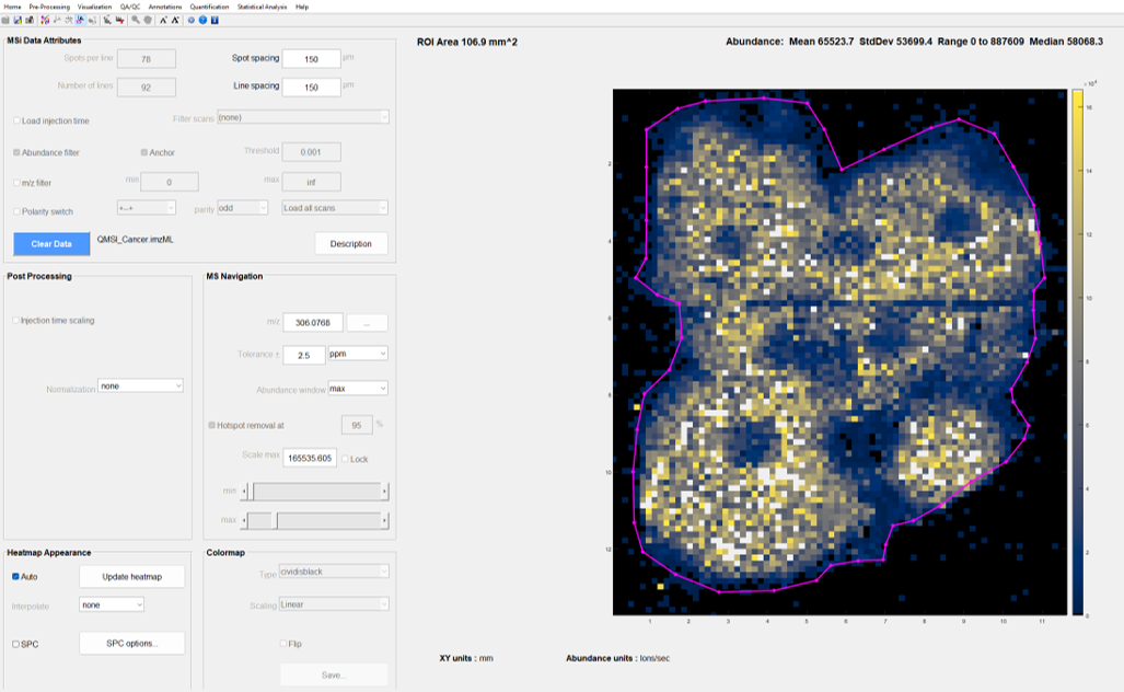
Figure 123: MSiReader GUI after loading a data set for quantification and drawing a ROI around the entire tissue.
Load a data set into MSiReader, adjust the spot and line spacing, select an m/z center value for the heatmap display and normalize to a reference peak (optional). The dataset must contain a spatial calibration curve deposited on the tissue. Select the polygon ROI tool and draw a region of interest (in this case, the entire tissue was selected). GUI is shown in Figure 123.
Next launch the quantification tool by selecting Absolute – QMSI spatial calibration curve from the drop-down menu under Quantification. The MSiQuantification GUI is shown below in Figure 124. It has edit boxes for entering the calibration parameters (density, thickness, calibration m/z and liquid volume), buttons for creating and removing ROIs around the calibration spots and edit boxes to enter a solution concentration for each ROI. The response treatment for calibration spots and the tissue ROI can be either the mean of the scan abundances or the sum of the abundances. Unit conversions can be calculated by typing arithmetic expressions in the edit boxes.
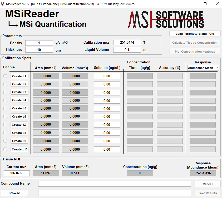
Figure 124: The MSiQuantification GUI.
The current m/z value in the Tissue ROI pane should be changed to the m/z of your internal standard to allow the user to draw the spots in the correct location (i.e., to make the spot scans “light up” in the heatmap). In this case, our internal standard has an m/z = 309.0797. The colorscale edit boxes and slider controls remain active in the MSiReader main GUI as well and can be adjusted to help reveal the calibration spots. In Figure 125 the max color scale slider has been lowered and six spots are clearly visible. There is a seventh spot with a zero-concentration solution amount.
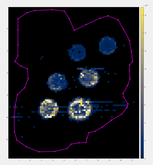
Figure 125: The m/z value has been changed in the Tissue ROI panel. The MSiReader colorscale and hot spot percentile were adjusted to increase the visibility of the internal standard spots.
Up to ten spot ROIs may be identified on the MSiReader heatmap. Clicking a Create L1, … button in the MSiQuantification GUI will switch window focus to the MSiReader window and enable the polygon drawing tool for the user to draw an ROI. The ROIs can be created in any order and moved and edited with the mouse. When the minimum number of ROIs for calibration have been drawn, the GUI is ready to calculate the tissue concentration. The default minimum number of spots is three, but this can be changed in the preferences INI file (§5) to a larger value. The corresponding spot solution amounts can be entered at any time and in any order. The enable/disable checkboxes can be used to see the effect of removing an “outlier” spot from the calculation without deleting it. The right-mouse context menu for each spot ROI contains an identifying label, e.g., L1, L2, L3, etc. In Figure 126 seven spots have been drawn; the 6 calibration points plus an ROI to represent the zero concentration.
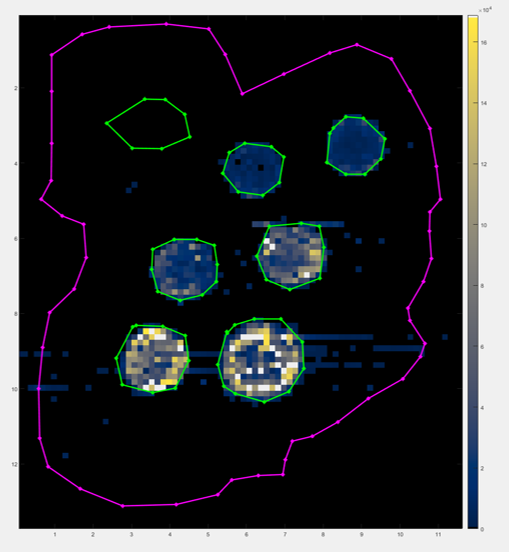
Figure 126: MSiReader after seven calibration spot ROIs have been drawn.
As an ROI is moved or edited, the area, volume and response values in the quantification table are updated automatically. If the liquid volume and solution concentration for an ROI has been entered, the tissue concentration is also calculated for the internal standard. After enough ROIs are complete and the solution concentrations (mg/mL) are entered, the MSiQuantification GUI will appear similar to
Figure 127 and the Calculate Tissue Concentration button will be enabled.
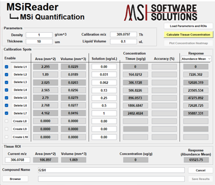
Figure 127: MSiQuantification GUI after drawing ROI spots and entering solution amounts.
Next change the Tissue ROI panel m/z value back to the correct value if it was changed in Step 2 (m/z = 306.0768 for this data set) and click the Calculate Tissue Concentration button. A linear regression of the spot response values (dependent variable) and their concentrations (independent variable) will be performed and the accuracy of the fit for each spot (100 minus percent error) calculated. The concentration in the Tissue ROI panel for the current m/z value can then be calculated from the slope and intercept of the regression line and the tissue ROI response. The GUI will update the tissue concentration as shown in Figure 128 (red circle).
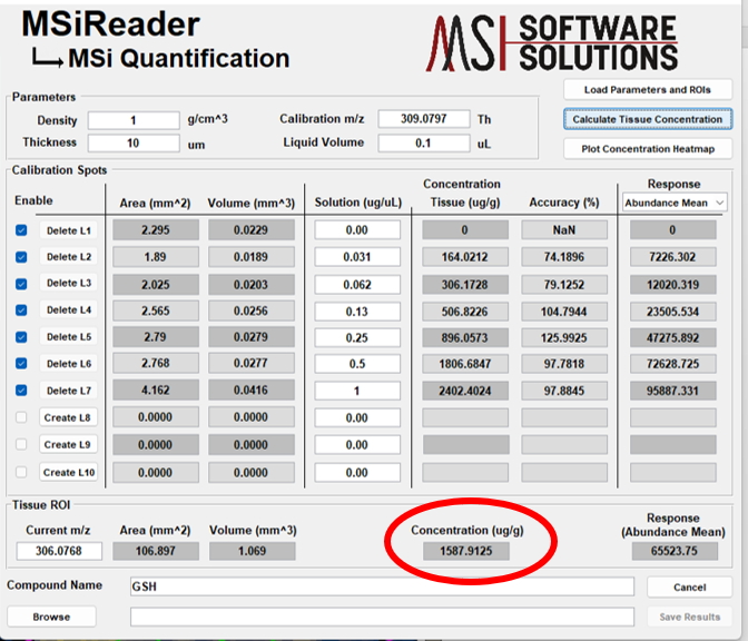
Figure 128: MSiQuantification results.
A plot of the regression results with 95% confidence limits is also displayed (see Figure 129) with the calibration spots shown as numbered red dots. The concentration vs. response point for the Tissue ROI is displayed as a magenta square labeled with the letter “T”. The regression equation and R2 value are displayed on the plot and the title contains the filename and any text that was entered in the Compound Name box.
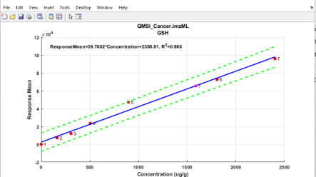
Figure 129: MSiQuantification linear regression result with 95% confidence limits.
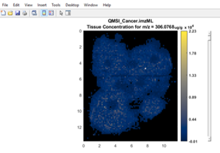
Figure 130: Heatmap plot using tissue concentration as the color scale.
In Figure 130 the data cursor toolbar icon, , can be used to identify the concentration and response corresponding to a point on the heatmap. Any number of data cursor tooltips can be added to the plot. The plot figure can be edited by the user and saved for publication. The default risk factor is 0.05. It can be changed in preferences INI file (§5) to any value between 0.68 and 0.001.
The Plot Concentration Heatmap button will display the full image heatmap in a new figure using the concentration calculated from the fit results as the color scale as shown in Figure 130.
The user can use the slider bar to the right of the heatmap to adjust the scale (see Figure 130). The concentrations are listed in mg/g. Click the Browse button to select an output file. Then the Save Results button will export the parameters and results of the quantification to an Excel workbook (or to text files if Excel is not installed) and a Matlab .mat file will also be saved (see Step 7 below). The Excel workbook will contain two worksheets: one with information about the data set (Error! Reference source not found.) and another with the regression parameters and results as well as the scan numbers for each calibration spot ROI and the Tissue ROI (Figure 131).
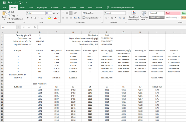
Figure 131: MSi Quantification results exported to Excel, regression worksheet.
The saved results MAT file can be used to reload the MSi Quantification parameters, spot and tissue ROIs, the tissue m/z, and normalization parameters in the same or a new MSiReader session. This allows the user to replicate an analysis on the same data set and get exactly the same result. To do this, click the button “Load Parameters and ROI’s” on the MSi Quantification GUI on the top right. (Figure 128). The user will be prompted if the data set name, its dimensions or other parameters do not match and given the opportunity to continue or cancel (Figure 132).
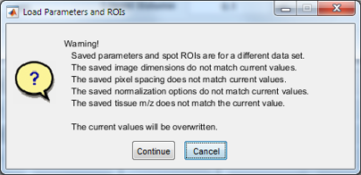
Figure 132: MSi Quantification load parameters dialog if loading incorrect .mat file.
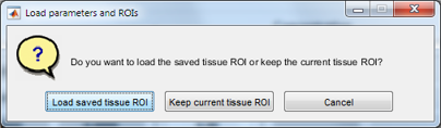
Figure 133: MSiQuantification tissue ROI dialog.
If the data sets do not match or the image dimensions are different continuing is likely to cause errors or produce meaningless results; however, it is permitted and could be a handy shortcut for analyzing multiple tissue samples with similar parameters. The ROIs can easily be “tweaked” and moved after they are automatically drawn. The user is also prompted to restore the Tissue ROI or keep the current ROI (Figure 133). Note that an ROI must be drawn somewhere on the tissue as described in Step 2 to enable the button that launches MSi Quantification.
7.7.3 Absolute – QMSI Voxel-by-Voxel Quantification
This approach to absolute quantification is where a tissue is mounted on a slide and then an internal standard of known concentration is sprayed on top of the slide / tissue at a known flow rate and total area covered. While this is a single point calibration curve, this approach significantly decreases variability from pixel-to-pixel (or voxel-to-voxel) due to tissue heterogeneity. An important point about this approach is some trial and error to determine the concentration required to have the ion abundance of the internal standard be as similar as possible to the ion abundance from the endogenous compound.
Figure 134: The V×V GUI for the absolute quantification of a targeted analyte.
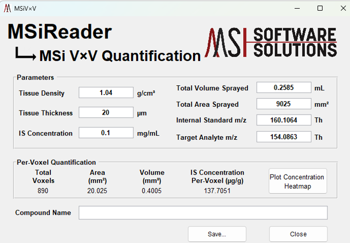 In this example, the spot spacing and line spacing were both 150 mm and the goal was to quantify dopamine (m/z = 154.0863) in the brain using stable isotope labeled dopamine m/z = 160.1064) as the internal standard. First, the user must use the polygon ROI tool and draw around the area that they wish to quantify the molecule of interest – in this case, dopamine. The GUI for the V×V quantification tool is shown in Figure 134. The values in the parameter box are all entered by the user based on the experimental conditions they used. Using these data and that from the ROI drawn by the user, the Per-Voxel Quantification information is calculated. The user can input the compound name (optional) if they want it displayed on top of the output images.
Once the experimental data is entered in, the user can click on Plot Concentration Heatmap. The GUI shown in Figure 135 is now displayed showing only the pixels (voxels) that were selected by the ROI tool. The user can click on any location and the coordinates, scan# and the absolute concentration will be displayed. The user can output the image from this GUI as well.
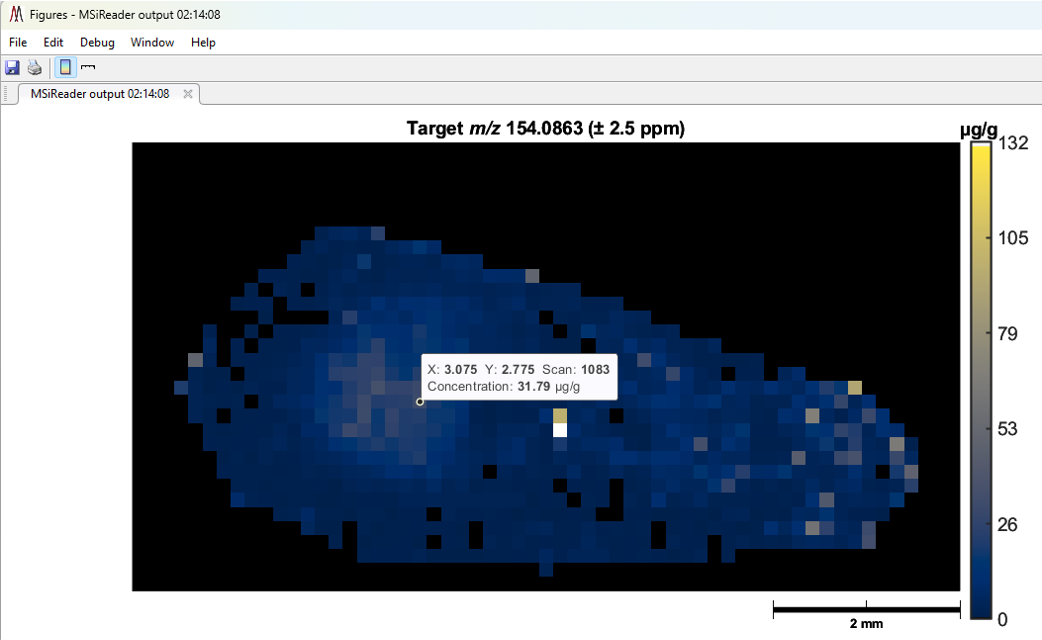
Figure 135: The interactive GUI which displays the concentration heatmap.
If the user would like to work up the data more, click on the Save button shown in the bottom of Figure 134. This will save in one worksheet the parameters of the experiment and in a second worksheet, more parameters and the concentration of the analyte by X,Y coordinates as well as scan number. This is a new tool in MSiReader and we are working on a statistical method to determine the error associated with each concentration and this will be added and explained in the near future.
7.7.4 Functional Mass Spectrometry Imaging PIE tool
In this section, the manual will provide a step-by-step example of how to use the Percent Isotope Enrichment (PIE) tool in MSiReader.

Figure 136: MSiReader after a fMSI dataset has been loaded into the main GUI.
After launching MSiReader, load an appropriate fMSI dataset as shown in Figure 136.
Note: If you don’t see this image using the test dataset from the www.msireader.com website, change the m/z value in the MS Navigation panel to 306.0765.
Normalize to the reference peak 320.0922. This is done in the main MSiReader GUI in the Post-Processing pane with the result shown in Figure 137. This is optional and depends on the experimental design.
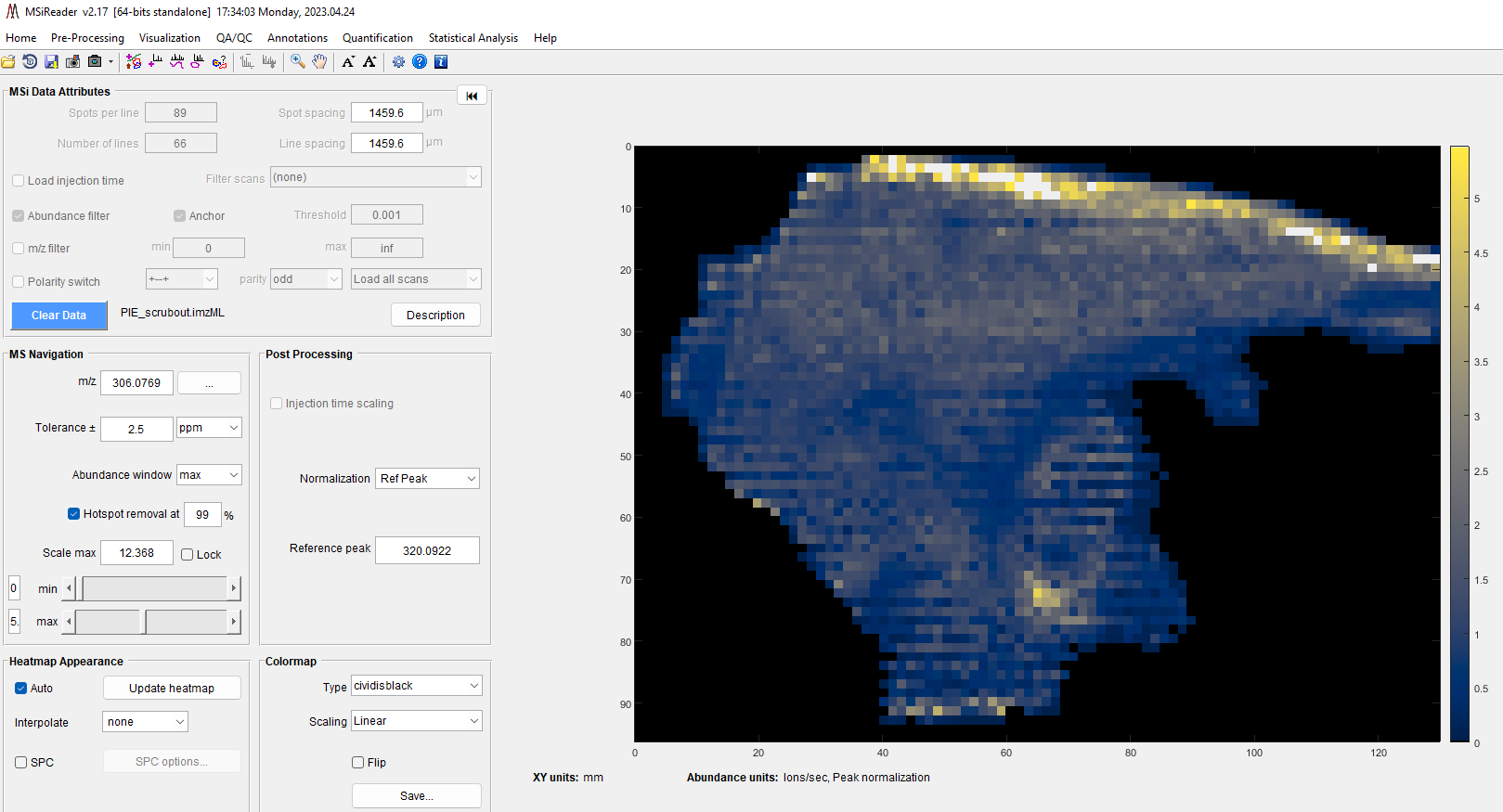
Figure 137: Heatmap after normalization to a compound that was homogenously coated across the entire sample.
Select the toolbar icon to enable the polygon tool and draw around the tissue. Save the ROI by right clicking on the heatmap and selecting Export ROI location info. In this way, you can reload the ROI for a future session and get the exact same ROI / result. Next, you can create a binary mask by right clicking on the magenta ROI line. Then choose scan scrubber under the pre-processing tools and remove pixels outside the ROI and then save the new imzML file (extension will add _scrubout) to the original filename. The area outside of the ROI will become black in the heatmap image.
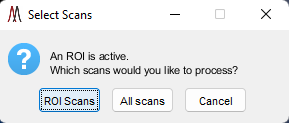
Figure 138: ROI selection dialog box when you launch the fMSI PIE Tool.
From the main menu, go to Quantification and then select fMSI PIE tool. Select ROI Scans in the dialog as shown in Figure 138.
The next step is to load an example matrix file. In this example, a file is provided with the filename Glutathione Probability Matrix (can be found in the test data sets at www.msireader.com). Then, select the worksheet from the dialog box that pops up.
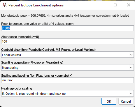
Figure 139: Options dialog box for the PIE tool. Leave the default settings as they are for this example. Heatmap color scaling options are shown in the GUI under “scaling and labeling”.
Once you chose the probability matrix, another dialog box will appear as shown in Figure 139. Leave the default options as they are and click the OK button.
Eight plots will automatically be produced. There are two plots for each m/z value in the isotopologues matrix: percent enrichment and normalized corrected abundance. The corrected abundance heatmap is normalized only if reference peak normalization is selected in MSiReader when the PIE tool is launched. Other normalization strategies are not supported. You can save each plot (heatmap) by using the menu bar in each plot.
A workbook will be also created and the user will automatically be prompted to choose a location and filename. It will contain five worksheets: Info, PIE Summary, PIE Abundance, PIE Abundance Normalized, and PIE Results. If normalization to a reference peak is not selected in MSiReader when the PIE tool is launched the PIE Abundance Normalized worksheet is not included in the results file.
7.8 Statistical Analysis of MSI Data
7.8.1 Preparing MSI Data for Statistical Analysis
A video tutorial on how to prepare MSI and HTS/phenotypic screening data for downstream statistical analysis can be found HERE.
An interactive multivariate analysis tool is provided in MSiReader. MSiPCA is based on singular value decomposition and loads an abundance matrix saved with the MSiExport sub-GUI, calculates PCA loadings and scores and plots the results for user selected components. The plots are 1) a heatmap showing the PCA score distribution for any number of user selected components (optional), 2) a biplot showing loading and scores for two or three components (and the end-user can select which PC’s to plot); and 3) an interactive PCA loadings plot as a function of m/z. The rows of the input matrix are observations (i.e., mass spectrometry scans, and the columns are variables, i.e., m/z values. The PCA results: component loadings, scores, latent variances, T-squared values, and explained variance percentages can be saved into a single Excel file, each in its own worksheet. Moreover, a scree plot is also automatically generated. Examples and more details will be shown later in this section.
Important Note: PCA algorithms are limited by the number of degrees of freedom (DOF) in the data you are working with; thus, if the # of scans (mass spectra) exceed the number of m/z values you can use all the m/z bins in the analysis. However, this is not typical with HRAM data and thus, the DOF will be limited to the number of scans in your data. In the PCA algorithm, it will use all the m/z binned data and then limit the output to those PC’s which describe most of the variance in the data and put in null values for m/z bins that exceed the number of DOF. Alternatively, prior to using the MSiPCA tool, the end-user can pre-process the data to bring the number of m/z values to be less than the number of scans. There are several ways to meet this criterion and more than one, or all of them, can be used. It depends on the types of data that the end-user is trying to analyze. The ways that the user can ensure that the # scans > # m/z values are listed here.
Select larger ROI’s for MSI data as this inherently increases the number of scans but, to a first approximation, the number of m/z values does not change.
Centroiding data. Since a profile peak contains many m/z values to describe the entire peak, by centroiding, one can reduce of m/z values in the dataset.
Abundance thresholding data. Given that each instrument is different in terms of the values it reports for ion abundance, the end-user should threshold the data so noise and low abundant peaks (high variance) are filtered out. This will substantially reduce the number of m/z values. It is recommended to set this value at an abundance that is 10× the limit-of-detection.
Filter out narrower m/z ranges prior to data export. Not recommended as a first approach because the goal of PCA and other multivariate methods is to use all the data that describes the data.
Below, an example is shown using a healthy tissue image and a cancerous tissue image where one ROI is drawn for each tissue and then the data is extracted using MSiExport.
Checking Data Attributes and Quality
It is important to check your data attributes and quality prior to selecting abundance threshold and the tolerance for peak exclusion. To check for the abundance threshold, the user should load a typical file in the study and then using the single pixel ROI, select an on-tissue pixel. Right click and “plot m/z spectrum”. Expand the spectrum using the mouse wheel and then look for low abundant peaks by moving the cursor on top of the peak. The pop-up window will give you the m/z value and the abundance. Look for the low abundance peaks and this will give the user an idea of what the threshold should be. In both the MSI and HCS data sets, the low abundance peaks are about 12,000 in ion abundance; thus, to be conservative the user could input 12,000 or to include additional lower abundance peaks, the user could use 8000.
The next step for QC would be to make a plot of the MMA for some representative data. The user can do this by loading a file and then going to the drop-down QA/QC menu and choosing “mass measurement accuracy”. In the main GUI, enter 10 ppm for starters into the tolerance and then make the plot. If the data is showing that it is all better than 5 ppm, then your tolerance for peak exclusion should be 5 ppm. If the data does not have the expected MMA and you have some known m/z values in the different images, the data should be mass corrected before doing anything else. This process can be found in §7.3.1.
Preparing data prior to using MSiPCA
Unload your data files from MSiReader.
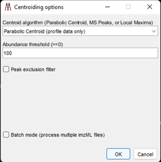
Figure 140: Centroid Data Options Panel in MSiReader
Launch the centroid data function under preprocessing drop-down menu. It will automatically be in batch mode since no data files are loaded. The dialogue box as shown in Figure 140 will appear. Once you set your parameters, click OK and it will open a file explorer to load the imzML files that you will use in the PCA.
If your dataset is profile data, it is recommended to centroid your data using the parabolic centroid. If the data is already centroided, please select local maxima in the drop-down menu. Next, select an abundance threshold that is specific to the instrument; 100 is the default but in most cases, this will be much higher.
Inevitability, mass spectrometry data has peaks in the mass spectra that are not sample related. For example, in MALDI, the ions from the organic matrix are present all over the tissue but are not tissue-specific. In ESI-post ionization methods and DESI, ambient molecules interact with the charged droplets and produce ambient background ions. The file PCAPeakstoRemove.txt has a single m/z that is not tissue specific; this file can be used in this example. It is critical that as many non-tissue specific ions for MSI and HCS data are removed from the data prior to PCA analysis because these could drive the PCA to an incorrect conclusion. See §7.3.4 for how to classify ions as being background or sample-specific. When peak exclusion filter is checked, the user can browse for .txt file containing the theoretical m/z values of the ions that are not sample related (make sure to include m/z values for ions with abundant A+1 and A+2 peaks). These will be excluded if the m/z is detected in the mass spectrum with a tolerance set by the end user. It is important to know the MMA of your dataset prior to setting this tolerance; otherwise, it will remove non-tissue peaks in some spectra that have high MMA but not in those that fall outside this tolerance. Click OK and new imzML files will be generated with “_centroided” automatically added to those files. If you loaded a *.raw file, the user can save the processed data as a *.mim file.
It is important to note that a user can also carry out the above steps for an entire folder of imzML files without ever having to load the files into MSiReader. To do this, clear the data and then choose Centroid Data under the Pre-Processing menu and enter in the dialogue box what function(s) needs to be carried out and click OK. It will then open a file explorer to choose the imzML files that need to be processed. Batch processing of *.raw files is not available but will be in a future release.
Exporting Data for Statistical Analysis using MSiExport
Open the processed data files that will be used to carry out PCA. Launch the MSiExport tool under the Annotations drop-down menu, then Data Export then Export Abundance Data. Draw a single ROI around all the data OR draw an interrogated and reference ROI. The user will be asked to select which scans to consider – select scans for the ROI(s). Next, choose Build and m/z list and bin the pixels in the ROI. Next, enter in values that correspond to your data; for high resolution accurate mass (HRAM) data, 5 ppm is recommended. Click the Browse button and enter a filename and folder for the .txt file to be prepared. Click OK. The .txt file will be the data that is entered into the PCA function.
For export to text format two files named <name>_info.txt and <name>_peaks.txt were saved. If the data was from a tiled image mosaic an additional file, <name>_files.txt was also saved. All of these are required to enable the full capabilities of MSiPCA and must be in the same folder. The <name>_peaks.txt file should be selected from the input dialog. While the user can use the *.csv file, we don’t recommend that as input to the multivariate tools in MSiReader but it is provided so users can use other software programs of their choice.
7.8.2 Principle Component Analysis (PCA)
A video tutorial on how to use the PCA tool can be found HERE.
7.8.2.1 Description of PCA
Principle Component Analysis (PCA) is a statistical technique used to simplify complex datasets by reducing the number of variables and retaining the most important information in a set of new, uncorrelated latent variables. PCA identifies the most important of these new variables or “principle components (PCs)” based on the amount variation they account for in a dataset. While there are as many PCs as there are original variables, the first PC accounts for the most variation in the data, the second accounts for the second most, etc., such that a small number of PCs may explain a large percentage of the overall variation found in the data. While the original variables may be heavily correlated, the resultant PCs are uncorrelated with one another.
PCA works by transforming the original variables into a new set of variables that are linear combinations of the originals. If variables are scaled (such that the variation of the variables is approximately equal), the value of a coefficient explains the impact that the original variable has on a PC. If a coefficient is extreme, the original variable is more highly correlated with that specific PC. This helps users identify which original variables are most important in explaining variation and potentially most important at differentiating between samples or groups.
PCA can be useful for analyzing mass spectrometry imaging data because it can help to identify the most important mass-to-charge ratios (m/z) in large datasets of spectral features. It can be useful for HCS data because in these cellular assays, the goal is to determine mode of action of different drugs. Both of these data types can be complex and high-dimensional with many variables representing different chemical components and their abundances. The number of m/z values, as well as correlation between scans and the identified peaks can make spectral datasets difficult to analyze directly. PCA can reduce the dimensionality of the datasets by converting the m/z values into smaller numbers of principle components that can explain large portions of the variation between scans. This is especially useful when comparing spectra from different samples and identifying similarities and differences between them. If PCs can be identified that separate samples or groups of samples, the chemical components that are responsible for the differences in PCs can be investigated.
7.8.2.2 PCA Details
Once samples are imported and ROI specified, PCA ready datasets are created. Each scan creates an observation with identified m/z values representing original variables and the abundances at each m/z value being the signal recorded for that variable. The m/z values are binned using a user defined range such that similar values across scans are labeled as the same m/z value (e.g., 212.0601 detected in one scan and 212.0603 detected in another may be binned together as the same m/z). The result is a set of scans with values recorded at each m/z found across all scans. If specific peaks were not identified in all scans, the observations missing these peaks are filled with 0’s for the missing values. Information about the sample, spatial location or well plate number of the scan, and possible group (e.g., treated vs. untreated, drug 1 vs. drug 2) are also retained.
Because variance in chemical abundances can be far greater at some m/z values than others, each m/z value is auto-scaled (mean centered and scaled by the standard deviation) prior to PCA, such that the mean and variance for each is approximately equal. Scaling m/z values is performed independently for each m/z and uses values from all scans and all samples.
Load the .txt file that was created in §7.8.1. A progress bar showing the loading of scans along with the total number of scans is shown. Principal component analysis is immediately performed when the OK button is clicked. The method used is singular value decomposition. As mentioned, prior to doing PCA, all the m/z measurements need to be on a similar abundance scale so that we can compare the variation attributed to each variable. Each m/z should be mean centered and scaled by the standard deviation. To accomplish this, the ion abundance is first converted to a scaled abundance (a*) for measurement i at a specific m/z:
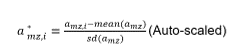
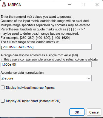
Figure 141: Selecting input columns by m/z range and abundance normalization (Z-score or Pareto). Checkboxes allow for individual heatmaps to be generated for each PC and an option to make a 3D plot.
where amz represents the vector of all abundances for that m/z.
Once all the scans are loaded into MSiReader, the dialogue box will appear as shown in Figure 141. This allows the user to select the full m/z range of the data or a narrower range(s). The user must then select abundance data normalization (Z-score or Pareto). The first checkbox is whether or not the end user wants to display individual heatmaps for each PC. We don’t recommend doing this as a default since datasets are quite large in the field. The second checkbox allow the user to change to a 3D biplot after the computations are done (PC1, PC2 and PC3 will be plotted).
Note: for two or more images, empty scans are inserted between the rows and columns to delineate the file boundaries and make the tilling pattern plaid. These scans are not removed before running the SVD so that the scan ordering and numbering of the data set as seen in the MSiReader heatmap plot is preserved. Instead, their abundance is set to NaN (not-a-number) and thus they are treated as missing data by the SVD algorithm and have no impact on the results.
As stated above, the PCA algorithm that is being used is MSiReader is SVD. It is important to note that when you have a n by p matrix of data, n being the rows (or scans) and p being the m/z values, the degrees of freedom are limited to n-1. Thus, if you load a data set with 500 mass spectra with each mass spectrum containing 100,000 m/z values, the maximum number of factors that can be returned is 499. When you have a wide (more columns than rows) matrix, PCA will calculate the covariance matrix of your input matrix first, resulting in a p by p covariance matrix. Next, the eigenvalue of the covariance matrix will be calculated. Since the input matrix is wide, the number of nonzero eigenvalues will not be larger than the degrees of freedom, which is n-1 in this case. Since the rest of the eigenvalues are zero, only the first n eigenvectors take part in the singular value decomposition, and the remainder being multiplied by zero. Only those eigenvectors not multiplied by zero are computed for decomposition and returned.
7.8.2.3 PCA Output Plots and Data
Loading the data and then running the MSiPCA tool will first prompt the user with how they would like the save the PCA results – this can be *.csv, *.txt or *.xlsx format. This saves the PCA scores data in an easy-to-use format for further analysis. Only the top 20 PC’s are exported.
Once the PCA data is saved, the default is to generate a 2D biplot; it is good to start with just the 2D biplot until you are more familiar with these. A 3D biplot can be selected if the checkbox in Figure 141 was selected.
The score plot is a representation of the dataset in the reduced dimensional space defined by one or more PCs. Scores from PCA represent the value of each PC for each observation. The score of a specific PC from a single scan is the linear combination of all m/z values recorded for that scan. A score plot displays these scores in 2 or 3-dimensional space with each point representing a single scan.
Each axis of the scores plot is a user chosen PC, such that two or three principle components can be viewed as a scatter plot. By default, the first principle component is displayed on x-axis and the second on the y-axis, though other PCs can be substituted by the user. Three-dimensional score plots plot the third PC on the z-axis. Scans with similar values for the displayed PCs are plotted near each other, whereas scans with largely different values for a PC are separated.
The score plot can be useful to identify patterns and relationships in the dataset. Clear separation between scans or samples can suggest that these principle components are capturing important differences between groups. If specific PCs are identified that differentiate between samples or scans, a loading plot can be used to detect the impact that each m/z value has on the PC.
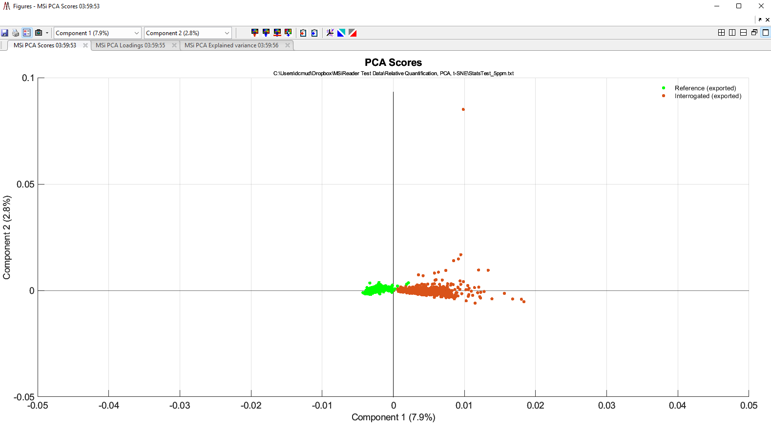
Figure 142: PCA of two small ROI’s derived from MSiExport of a healthy and a cancer tissue.
An example of a two-dimensional biplot is shown in Figure 142 and will appear automatically. Note that the observations from each file in the data set are assigned the same color (in this case, red is ovarian cancer tissue and green is healthy ovary tissue). The colors are automatically selected by MSiPCA from the default plot color order if there are fewer than eight files or from a random permutation of the current colormap if there are more than seven files. The data cursor, rotate, pan and zoom tools are to the upper right of the plot and will appear after the mouse is hovered over the plot for a few seconds.
The observation data cursor display text has been customized to include the scan location for an observation in the image mosaic and in the original file. The variable data cursor display text shows the m/z value. The component values are also shown in both types of data cursor text.
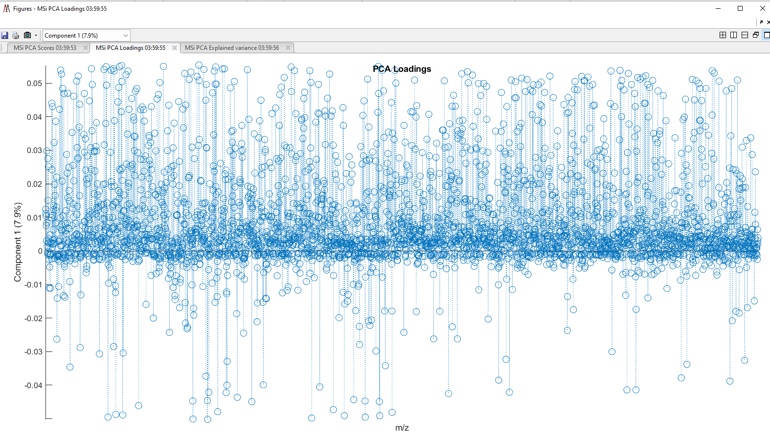
Figure 143: PCA Loadings Plot for the data shown in Figure 142.
Note that at the top of Figure 142, Component 1 and Component 2 are listed with their amount of explained variance. These are drop down windows and the end-user can then make plots of PC1 versus PC3 for example, and so on. Also note there are two other tabs, one is PCA loadings plot (Figure 143) and the other is a scree plot ().
The loadings plot is a graphical representation of the relationship between the mass-to-charge ratios and the resultant principle components. Each of the original m/z values has a loading for each PC, representing that m/z’s coefficient from the linear combination of all m/z. A loading that is high relative to others indicate that a strong positive correlation between abundances at that m/z and the PC, whereas loadings that are low compared to others represent strong negative correlation.
For loadings plot, a PC is chosen by the user. The x-axis contains each m/z (or possibly a subset of m/z’s if filtered) detected in the dataset. The y-axis contains the coefficient associated with that m/z value for the PC.
If one or more PCs are identified that separate or describe the data well, the loadings plot can help identify the mass-to-charge ratios that have the highest impact on these PCs.
The PCA loadings plot (Figure 143), one can use the mouse wheel to expand and contract the x-axis and the cursor will indicate which m/z value describes that particular loading for PC1. Note that the upper left-hand corner, the user can select which PCA loadings plot they want. It is a pull-down menu and also indicates the percentage of explained variance.
The scree plot for the data is shown in Figure 144. Note that the number of principal components is limited to 2077 since only 2078 scans were used to generate this test dataset.
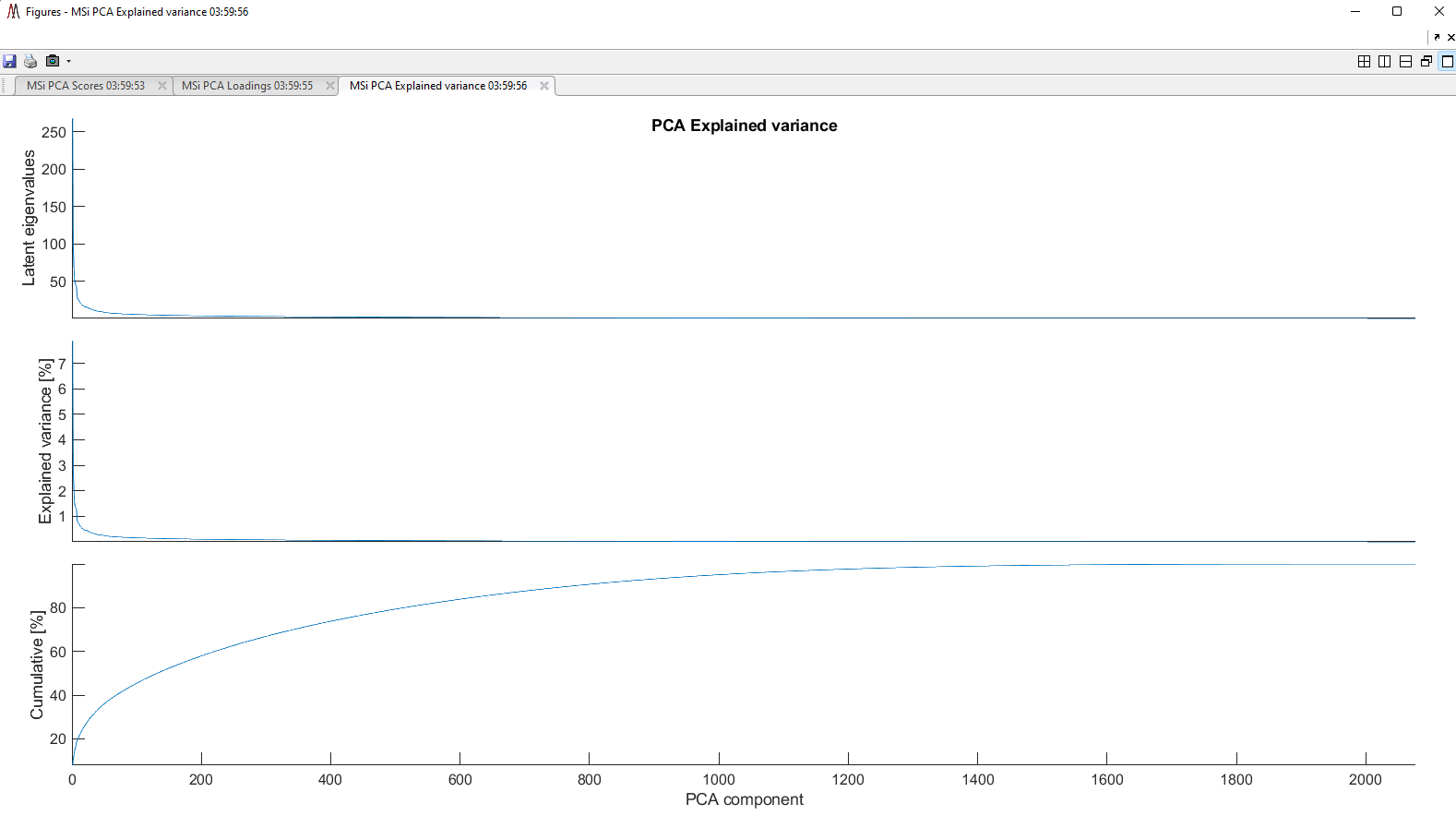
Figure 144: Scree plot for the data shown in Figure 142
Four icons are on the biplot toolbar; the function of each icon is described below.
The m/z values for all current variable data cursors are appended to the clipboard. The icon is always enabled on the biplot toolbar.
The scan numbers for all data cursors attached to an observation are appended to the clipboard. The icon is enabled when the observation scores are plotted.
Visibility of observation scan markers on the biplot is toggled. The icon is enabled when the observation scores are plotted. If the data set is for a folder of files, a selection dialog is launched with an entry for each file. Markers for the de-selected files are hidden on the biplot. Any data cursor text boxes attached to these scans are also hidden but not deleted. Click the icon again to restore the hidden markers and data cursors.
 Takes the average of all scores for each sample type. In this case there are only two samples and thus, plotting all of the data (each voxel is a point for each sample) made more visual sense.
The text files or the single Excel file with multiple worksheets also contain important information about the PCA analysis – please export these values using the *.txt or *.xlsx format while the *.csv format only includes the scores for further downstream analysis using other programs.
pca_mz:
A list of the m/z values identified across all scans and used for PCA.
pca_scores:
The scores for all observations and all PCs. Each row represents a scan and columns represent the score for each PC.
pca_coeff:
The loadings (coefficients) for each m/z value on the principle components. Each row represents an original variable (m/z) and each column represents a PC. The score of a specific PC is determined by multiplying each coefficient by the abundance for the associated m/z and summing these across all m/z’s.
pca_latent:
The eigenvalue associated with each PC. This represents the total amount of variation in that dataset that is explained by each PC on its original scale.
pca_varpct:
The percentage of variation of the data described by each PC. This is determined by dividing each of the values in pca_latent by the sum of all values.
pca_tsquare:
A list of Hotelling t-squared values from each observation. These measure the distance that each observation is from the center of the dataset based on the principle components. High t-squared values can indicate that an observation is far away from the center of the dataset and may be an outlier.
7.8.3 t-distributed Stochastic Neighbor Embedding (t-SNE)
A video tutorial on how to use the t-SNE tool can be found HERE.
7.8.3.1
Similar to PCA, t-SNE is used to understand high-dimensional data and visualize it in lower-dimensional spaces. While PCA is a useful tool to analyze datasets with linear relationships between variables, t-SNE is a dimensionality reduction tool that relaxes these assumptions and can project linearly non-separable data into reduced dimensions. Please make sure you read through §7.8.1 to make sure your data is properly prepared prior to using this statistical tool.
t-SNE works by constructing a probability distribution for pairs of observations of high dimensions (many m/z values) such that observations that are similar have a relative high probability assigned and observations that are dissimilar have low probabilities assigned. This probability distribution incorporates all m/z values found across a dataset. A second probability distribution is created in lower dimensional space (typically 2 or 3 dimensions). The observations are adjusted in the low-dimensional space so that the second probability distribution matches the first probability distribution as closely as possible. This allows visualization of complex, high-dimensional datasets in lower dimensional space while preserving the underlying structure of the dataset (similarities and differences between scans or samples).
7.8.3.3 t-SNE Details
Once samples are imported and ROI specified, t-SNE ready datasets are created. Each scan creates an observation with identified m/z’s representing original variables and the abundances at each m/z value being the values recorded for that variable. The m/z values are binned using a user defined range such that similar values across scans are labeled as the same m/z value (e.g., 212.0601 detected in one scan and 212.0603 detected in another may be binned together as the same m/z). The result is a set of scans with values recorded at each m/z found across all scans. If specific peaks were not identified in all scans, the observations missing these peaks are filled with 0’s for the missing m/z’s. Information about the sample, spatial location of the scan, and possible group (e.g., treated vs. untreated) are also retained.
Because variance in chemical abundances can be far greater at some m/z values than others, each m/z value is auto-scaled (mean centered and scaled by the standard deviation) prior to t-SNE, such that the mean and variance for each is approximately equal. Scaling m/z values is performed independently for each m/z and uses values from all scans and all samples.
Next the t-SNE algorithm is applied to generate observations in lower dimensionality. Pairwise similarities are determined between each pair of scans based on the distance measure chosen (e.g., Euclidian distance). This similarity is represented as the conditional probability that a pair are neighbors in the high-dimensional space (i.e., high probability indicates scans are similar whereas low probability indicates significant differences between scans). A probability distribution is constructed based on all pairwise similarities in the high-dimensional space, using a Gaussian kernel to define each probability.
Next, a similar probability distribution is constructed in a lower dimensional space and using a Students-t kernel. Observations are initially scattered at random in the lower dimensional space. The lower dimension distribution is then optimized by minimizing the Kullback-Leiber divergence between the higher and lower dimensional distributions. Points are adjusted such that observations that are similar in higher dimensions are also similar in the lower dimension distribution.
7.8.3.3 Input and Output for t-SNE
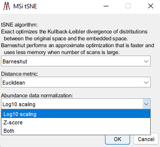
Figure 145: t-SNE dialog box. It is recommended that Barneshut and Euclidean (defaults) are used but other options are available in the pull-down menus. Choose the scaling function (Log10, Z-score or Both which is Log10 followed by Z-score). t-SNE can also make use of a seeding function which will change the plots. To use the seeding function, check the box re-randomize (not visible) so that each time you process the file, a different set of random seed functions are applied.
The input for t-SNE is the same as for MSiPCA. Launch t-SNE by going to the menu Statistical Analysis and then select t-SNE. When the tool is launched, a file explorer will open asking the end-user to select a .txt file to load. In this example, it is the same .txt file that was used for MSiPCA. Load the .txt file – a progress bar will appear showing the user the scan number being loaded (e.g., 1000 out of 5069) and a percentage of the total number of scans. Next, the dialogue box shown in Figure 145 will be displayed. Please see figure caption for the choices that the user can make. While the computations are being carried out, a window is displayed indicating “Computing tSNE may take some time, please be patient”.
The user will be prompted to save the tSNE output data (scan number, source, DIM1 and DIM2) for the analysis in either *.csv format or *.xlsx format. Choose which option and where the data file should be stored.
MSiReader’s t-SNE algorithm generates a 2-dimensional plot of the dataset with a single point for each scan. The units and scale of these dimensions are unimportant as they do not directly correspond the units of the original dataset. Instead, the relationship and relative distances between points can be observed. Points that are close to one another are more similar in high-dimensional space. Clusters of points may identify similar data points in high dimensions, where the more tightly points are clustered, the more similar the abundances detected at each m/z are among scans.
Data points can be colored based on sample or group (e.g., Treated vs. Untreated). Clear clustering based on these criteria indicate that the dataset can be separated based on some set of m/z values. Plots may also identify other important clusters or relationships such as similar sample types (e.g., type of tissue being scanned) or outliers that can be removed by redefining the ROI.
t-SNE can identify non-linear relationships between scans in high-dimensional space and help determine if data points can be clustered or separated. However, the reduced dimensions do not have a defined relationship with the original variables making interpretation of variables that are important difficult. If relationships or clusters are identified using t-SNE, alternative analytical methods should be used to further investigate variables responsible.
When the t-SNE computations have been completed, a plot of t-SNE Dimension 1 (x-axis) and t-SNE Dimension 2 (y-axis) are displayed as shown in Figure 146.
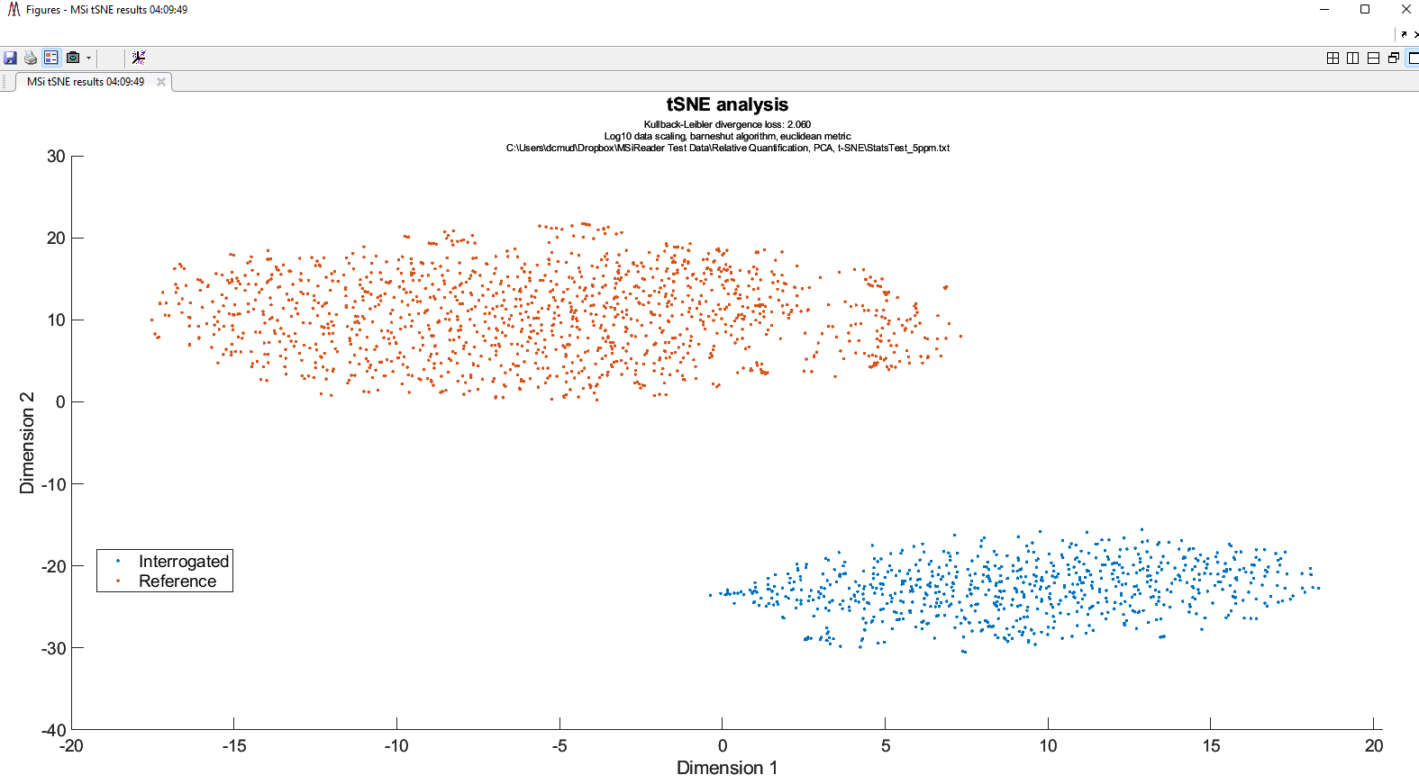
Figure 146: t-SNE 2D output plot. Clearly, the cancer and healthy samples separate well using this multivariate approach. Notice that on the top, the choices the user made are listed under t-SNE analysis.
7.8.4 Volcano Plot
7.8.4.1 Preparing your data
Load all of the data into MSiReader into the main GUI. Use filenames that will be easy to tell which ones are treatment / disease and which ones are controls. The end user should have already generated a m/z list of peaks – for example, using a Metaspace annotation file or a data export using MSiSpectrum. Once you have your m/z list, launch MSiExport (under annotations menu) and it will prompt user to select ROI scans (if you selected an ROI) or All Scans. Next, select a file containing a list of m/z values. It will prompt the user to select a file (single column of data that contains a list of m/z values). MSiReader will check the file to make sure it is allowed and then it will display the number of m/z values that were found. Finally, select the folder and filename where the output data file will go. Click OK.
Note: Given that not all data that is collected used an arbitrary ROI, one option is to load each file, scrub out the pixels that are not related to the tissue, and then save new imzML files. Since MSiReader will ignore the “zeros” in the scrubbed file, downstream analysis will not be affected. Load these scrubbed files into MSiReader at the same time, and then go to the MSiExport and follow directions above. This will generate a file of m/z values and abundances that can be used for the Volcano Plot.
Related to this, if your project has treatment / disease and control in a single tissue image, you can go in, draw an ROI around the region containing the diseased tissue and then scrub out the remaining data. The data is saved as a new imzML file. Do the same for the control regions of that same tissue image starting by re-loading the original data. Save that as a new imzML file. You can also save the ROI’s for each selection you have made so if you need to, you can go back and recall these, so you don’t have to remember the details of the ROI that you chose.
Note: A volcano plot requires at least two images for control and two images for treatment/disease. Two images are needed for each group in order to generate a p-value and fold-change for each m/z value – thus, a minimum of 4 samples being measured.
7.8.4.2 Generate the Volcano Plot
Figure 147 shows the sub-GUI where the end-user will load their data. This is the file the
Figure 147: MSiVolcano load file sub-GUI. Click ‘Browse”. Choose the data export file from File Explorer and then Click “OK”.
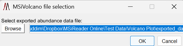
end user created above using the MSiExport tool. Once you load the file and click “OK”, another sub-GUI will appear as shown in Figure 148.
Figure 148: MSiVolcano – assign each file as either “Control” or “Treatment” by the pull-down menus after each file name. Once those are correct, click “OK”.
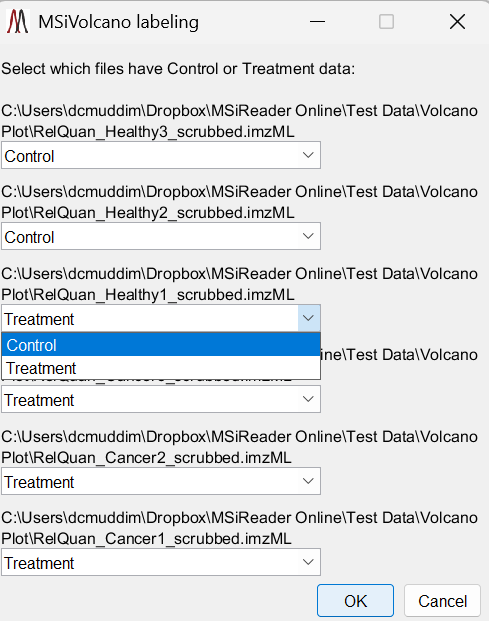
Figure 149 shows the output of the volcano plot which is a plot of -log10 p-value versus log2 fold-change. We also provide a table of the results which includes m/z, p-value, and fold change. At the bottom of the plot, the end-user can change the fold-change and the p-value. One can also export their data into an Excel spreadsheet and continue to work up the data using the Export function at the bottom of the table.
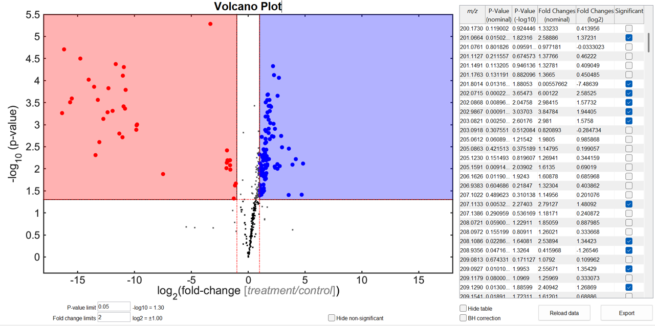
Figure 149: After the end-user clicks “OK” from the sub-GUI in Figure 148, a Volcano plot and a data table will appear as shown here. To export just the volcano plot, check the “hide table” toggle and then use the camera icon on the top left of the plot to export to the figure in numerous different file formats.
There are other options in the Volcano plot using the checkboxes along the bottom of the GUI. The end-user can change the p-value limit and/or the fold-change by entering those values in. If the user would like to plot and tabulate only the significant values, the user can check the “hide non-significant” box. If the user would like to decrease the false-discovery rate, the end user can check the BH correction box – this correction is the Benjamini-Hochberg correction.
The user can unhide the table of data and from there, the user can export that data for loading into other programs such as Excel, R, etc. When the BH is checked, the plot and table automatically update with the corrected data. Likewise, when the box is unchecked, the plot and table will update automatically again.
If you click and hold down your mouse on the plot, the user can move it around to their liking and the output figure will contain those choices. The x- and y-labels as well as the title can be clicked on and changed to the user’s preference before exporting the figure.